| Issue |
A&A
Volume 695, March 2025
|
|
|---|---|---|
| Article Number | A233 | |
| Number of page(s) | 21 | |
| Section | Extragalactic astronomy | |
| DOI | https://doi.org/10.1051/0004-6361/202452600 | |
| Published online | 24 March 2025 | |
A multifrequency study of sub-parsec jets with the Event Horizon Telescope
1
Max-Planck-Institut für Radioastronomie, Auf dem Hügel 69, D-53121 Bonn, Germany
2
Instituto de Astrofísica de Andalucía-CSIC, Glorieta de la Astronomía s/n, E-18008 Granada, Spain
3
Astronomy Department, Universidad de Concepción, Casilla 160-C, Concepción, Chile
4
Korea Astronomy and Space Science Institute, Daedeok-daero 776, Yuseong-gu, Daejeon 34055, Republic of Korea
5
Massachusetts Institute of Technology Haystack Observatory, 99 Millstone Road, Westford, MA 01886, USA
6
Black Hole Initiative at Harvard University, 20 Garden Street, Cambridge, MA 02138, USA
7
Center for Astrophysics | Harvard & Smithsonian, 60 Garden Street, Cambridge, MA 02138, USA
8
Steward Observatory and Department of Astronomy, University of Arizona, 933 N. Cherry Ave., Tucson, AZ 85721, USA
9
Data Science Institute, University of Arizona, 1230 N. Cherry Ave., Tucson, AZ 85721, USA
10
Program in Applied Mathematics, University of Arizona, 617 N. Santa Rita, Tucson, AZ 85721, USA
11
NASA Hubble Fellowship Program, Einstein Fellow, USA
12
Department of Astrophysics, Institute for Mathematics, Astrophysics and Particle Physics (IMAPP), Radboud University, P.O. Box 9010 6500 GL Nijmegen, The Netherlands
13
Institute of Astronomy and Astrophysics, Academia Sinica, 645 N. A’ohoku Place, Hilo, HI 96720, USA
14
Department of Physics and Astronomy, University of Hawaii at Manoa, 2505 Correa Road, Honolulu, HI 96822, USA
15
Leiden Observatory, Leiden University, Postbus 2300, 9513 RA, Leiden, The Netherlands
16
Netherlands Organisation for Scientific Research (NWO), Postbus 93138, 2509 AC Den Haag, The Netherlands
17
Aalto University Department of Electronics and Nanoengineering, PL 15500, FI-00076 Aalto, Finland
18
Aalto University Metsähovi Radio Observatory, Metsähovintie 114, FI-02540 Kylmälä, Finland
19
National Radio Astronomy Observatory, 520 Edgemont Road, Charlottesville, VA 22903, USA
20
Department of Space, Earth and Environment, Chalmers University of Technology, Onsala Space Observatory, SE-43992 Onsala, Sweden
21
Shanghai Astronomical Observatory, Chinese Academy of Sciences, 80 Nandan Road, Shanghai 200030, People’s Republic of China
22
Instituto de Astronomia, Geofísica e Ciências Atmosféricas, Universidade de São Paulo, R. do Matão, 1226, São Paulo, SP 05508-090, Brazil
23
Dipartimento di Fisica, Universitá degli Studi di Cagliari, SP Monserrato-Sestu km 0.7, I-09042 Monserrato (CA), Italy
24
INAF – Osservatorio Astronomico di Cagliari, via della Scienza 5, I-09047 Selargius (CA), Italy
25
INFN, sezione di Cagliari, I-09042 Monserrato (CA), Italy
26
Instituto de Física, Pontificia Universidad Católica de Valparaíso, Casilla 4059, Valparaíso, Chile
27
Independent researcher
28
Department of Astronomy, University of Illinois at Urbana-Champaign, 1002 West Green Street, Urbana, IL 61801, USA
29
National Astronomical Observatory of Japan, 2-21-1 Osawa, Mitaka,Tokyo 181-8588, Japan
30
Departament d’Astronomia i Astrofísica, Universitat de Valéncia, streetC. Dr. Moliner 50 E-46100 Burjassot, Valéncia, Spain
31
Department of Physics, Faculty of Science, Universiti Malaya, 50603 Kuala Lumpur, Malaysia
32
Department of Physics & Astronomy, The University of Texas at San Antonio, One UTSA Circle, San Antonio, TX 78249, USA
33
Institute of Astronomy and Astrophysics, Academia Sinica, 11F of Astronomy-Mathematics Building, AS/NTU No. 1, Sec. 4, Roosevelt Rd., Taipei 106216, Taiwan, R.O.C.
34
Observatori Astronómic, Universitat de Valéncia, C. Catedrático José Beltrán 2, E-46980 Paterna, Valéncia, Spain
35
Yale Center for Astronomy & Astrophysics, Yale University, 52 Hillhouse Avenue, New Haven, CT 06511, USA
36
Department of Physics, University of Illinois, 1110 West Green Street, Urbana, IL 61801, USA
37
Fermi National Accelerator Laboratory, MS209, P.O. Box 500 Batavia, IL 60510, USA
38
Department of Astronomy and Astrophysics, University of Chicago, 5640 South Ellis Avenue, Chicago, IL 60637, USA
39
East Asian Observatory, 660 N. A’ohoku Place, Hilo, HI 96720, USA
40
James Clerk Maxwell Telescope (JCMT), 660 N. A’ohoku Place, Hilo, HI 96720, USA
41
California Institute of Technology, 1200 East California Boulevard, Pasadena, CA 91125, USA
42
Institut de Radioastronomie Millimétrique (IRAM), 300 rue de la Piscine, F-38406 Saint Martin d’Hères, France
43
Perimeter Institute for Theoretical Physics, 31 Caroline Street North, Waterloo ON N2L 2Y5, Canada
44
Department of Physics and Astronomy, University of Waterloo, 200 University Avenue West, Waterloo ON N2L 3G1, Canada
45
Waterloo Centre for Astrophysics, University of Waterloo, Waterloo ON N2L 3G1, Canada
46
Department of Astronomy, University of Massachusetts, Amherst, MA 01003, USA
47
University of Science and Technology, Gajeong-ro 217, Yuseong-gu, Daejeon 34113, Republic of Korea
48
Kavli Institute for Cosmological Physics, University of Chicago, 5640 South Ellis Avenue, Chicago, IL 60637, USA
49
Department of Physics, University of Chicago, 5720 South Ellis Avenue, Chicago, IL 60637, USA
50
Enrico Fermi Institute, University of Chicago, 5640 South Ellis Avenue, Chicago, IL 60637, USA
51
Princeton Gravity Initiative, Jadwin Hall, Princeton University, Princeton, NJ 08544, USA
52
Cornell Center for Astrophysics and Planetary Science, Cornell University, Ithaca, NY 14853, USA
53
Key Laboratory of Radio Astronomy and Technology, Chinese Academy of Sciences, A20 Datun Road, Chaoyang District Beijing 100101, People’s Republic of China
54
Department of Astronomy, Yonsei University, Yonsei-ro 50, Seodaemun-gu, 03722 Seoul, Republic of Korea
55
Physics Department, Fairfield University, 1073 North Benson Road, Fairfield, CT 06824, USA
56
Instituto de Astronomía, Universidad Nacional Autónoma de México (UNAM), Apdo Postal 70-264, Ciudad de México, Mexico
57
Institut für Theoretische Physik, Goethe-Universität Frankfurt, Max-von-Laue-Straße 1, D-60438 Frankfurt am Main, Germany
58
Research Center for Astronomical Computing, Zhejiang Laboratory, Hangzhou 311100, People’s Republic of China
59
Tsung-Dao Lee Institute, Shanghai Jiao Tong University, Shengrong Road 520, Shanghai 201210, People’s Republic of China
60
Department of Astronomy and Columbia Astrophysics Laboratory, Columbia University, 500 W. 120th Street, New York, NY 10027, USA
61
Center for Computational Astrophysics, Flatiron Institute, 162 Fifth Avenue, New York, NY 10010, USA
62
Dipartimento di Fisica “E. Pancini”, Universitá di Napoli “Federico II”, Compl. Univ. di Monte S. Angelo, Edificio G, Via Cinthia, I-80126 Napoli, Italy
63
INFN Sez. di Napoli, Compl. Univ. di Monte S. Angelo, Edificio G, Via Cinthia, I-80126 Napoli, Italy
64
Wits Centre for Astrophysics, University of the Witwatersrand, 1 Jan Smuts Avenue, Braamfontein, Johannesburg 2050, South Africa
65
Department of Physics, University of Pretoria, Hatfield, Pretoria 0028, South Africa
66
Centre for Radio Astronomy Techniques and Technologies, Department of Physics and Electronics, Rhodes University, Makhanda 6140, South Africa
67
ASTRON, Oude Hoogeveensedijk 4, 7991 PD Dwingeloo, The Netherlands
68
LESIA, Observatoire de Paris, Université PSL, CNRS, Sorbonne Université, Université de Paris, 5 place Jules Janssen, F-92195 Meudon, France
69
JILA and Department of Astrophysical and Planetary Sciences, University of Colorado, Boulder, CO 80309, USA
70
National Astronomical Observatories, Chinese Academy of Sciences, 20A Datun Road, Chaoyang District Beijing 100101, PR China
71
Las Cumbres Observatory, 6740 Cortona Drive, Suite 102, Goleta, CA 93117-5575, USA
72
Department of Physics, University of California, Santa Barbara, CA 93106-9530, USA
73
Department of Electrical Engineering and Computer Science, Massachusetts Institute of Technology, 32-D476, 77 Massachusetts Ave., Cambridge, MA 02142, USA
74
Google Research, 355 Main St., Cambridge, MA 02142, USA
75
Institut für Theoretische Physik und Astrophysik, Julius-Maximilian-Universität Würzburg, Emil-Fischer-Straße 31, 97074 Würzburg, Germany
76
Department of History of Science, Harvard University, Cambridge, MA 02138, USA
77
Department of Physics, Harvard University, Cambridge, MA 02138, USA
78
NCSA, University of Illinois, 1205 W. Clark St., Urbana, IL 61801, USA
79
Institute for Mathematics and Interdisciplinary Center for Scientific Computing, Heidelberg University, Im Neuenheimer Feld 205, Heidelberg 69120, Germany
80
Institut für Theoretische Physik, Universität Heidelberg, Philosophenweg 16, 69120 Heidelberg, Germany
81
CP3-Origins, University of Southern Denmark, Campusvej 55, 5230 Odense, Denmark
82
Instituto Nacional de Astrofísica, Óptica y Electrónica. Apartado Postal 51 y 216, 72000 Puebla Pue., Mexico
83
Consejo Nacional de Humanidades, Ciencia y Tecnología, Av. Insurgentes Sur 1582, 03940 Ciudad de México, Mexico
84
Key Laboratory for Research in Galaxies and Cosmology, Chinese Academy of Sciences, Shanghai 200030, People’s Republic of China
85
Mizusawa VLBI Observatory, National Astronomical Observatory of Japan, 2-12 Hoshigaoka, Mizusawa, Oshu, Iwate 023-0861, Japan
86
Department of Astronomical Science, The Graduate University for Advanced Studies (SOKENDAI), 2-21-1 Osawa, Mitaka, Tokyo 181-8588, Japan
87
Department of Physics, McGill University, 3600 rue University, Montréal QC H3A 2T8, Canada
88
Trottier Space Institute at McGill, 3550 rue University, Montréal QC H3A 2A7, Canada
89
NOVA Sub-mm Instrumentation Group, Kapteyn Astronomical Institute, University of Groningen, Landleven 12, 9747 AD Groningen, The Netherlands
90
Department of Astronomy, School of Physics, Peking University, Beijing 100871, People’s Republic of China
91
Kavli Institute for Astronomy and Astrophysics, Peking University, Beijing 100871, People’s Republic of China
92
Department of Astronomy, Graduate School of Science, The University of Tokyo, 7-3-1 Hongo, Bunkyo-ku, Tokyo 113-0033, Japan
93
The Institute of Statistical Mathematics, 10-3 Midori-cho, Tachikawa, Tokyo 190-8562, Japan
94
Department of Statistical Science, The Graduate University for Advanced Studies (SOKENDAI), 10-3 Midori-cho, Tachikawa, Tokyo 190-8562, Japan
95
Kavli Institute for the Physics and Mathematics of the Universe, The University of Tokyo, 5-1-5 Kashiwanoha, Kashiwa 277-8583, Japan
96
ASTRAVEO LLC, PO Box 1668 Gloucester MA 01931, USA
97
Applied Materials Inc., 35 Dory Road, Gloucester MA 01930, USA
98
Institute for Astrophysical Research, Boston University, 725 Commonwealth Ave., Boston, MA 02215, USA
99
Institute for Cosmic Ray Research, The University of Tokyo, 5-1-5 Kashiwanoha, Kashiwa, Chiba 277-8582, Japan
100
Joint Institute for VLBI ERIC (JIVE), Oude Hoogeveensedijk 4, 7991 PD Dwingeloo, The Netherlands
101
Department of Physics, Ulsan National Institute of Science and Technology (UNIST), 50 UNIST-gil, Eonyang-eup, Ulju-gun, Ulsan 44919, Republic of Korea
102
Department of Physics, Korea Advanced Institute of Science and Technology (KAIST), 291 Daehak-ro, Yuseong-gu, Daejeon 34141, Republic of Korea
103
Kogakuin University of Technology & Engineering, Academic Support Center, 2665-1 Nakano, Hachioji, Tokyo 192-0015, Japan
104
Graduate School of Science and Technology, Niigata University, 8050 Ikarashi 2-no-cho, Nishi-ku, Niigata 950-2181, Japan
105
Physics Department, National Sun Yat-Sen University, No. 70, Lien-Hai Road, Kaosiung City 80424, Taiwan, R.O.C.
106
National Optical Astronomy Observatory, 950 N. Cherry Ave., Tucson, AZ 85719, USA
107
Department of Physics, The Chinese University of Hong Kong, Shatin, N. T., Hong Kong
108
School of Astronomy and Space Science, Nanjing University, Nanjing 210023, People’s Republic of China
109
Key Laboratory of Modern Astronomy and Astrophysics, Nanjing University, Nanjing 210023, People’s Republic of China
110
INAF-Istituto di Radioastronomia, Via P. Gobetti 101, I-40129 Bologna, Italy
111
INAF-Istituto di Radioastronomia & Italian ALMA Regional Centre, Via P. Gobetti 101, I-40129 Bologna, Italy
112
Department of Physics, National Taiwan University, No. 1, Sec. 4, Roosevelt Rd., Taipei 106216, Taiwan, R.O.C
113
Instituto de Radioastronomía y Astrofísica, Universidad Nacional Autónoma de México, Morelia 58089, Mexico
114
David Rockefeller Center for Latin American Studies, Harvard University, 1730 Cambridge Street, Cambridge, MA 02138, USA
115
Yunnan Observatories, Chinese Academy of Sciences, 650011 Kunming, Yunnan Province, People’s Republic of China
116
Center for Astronomical Mega-Science, Chinese Academy of Sciences, 20A Datun Road, Chaoyang District, Beijing 100012, People’s Republic of China
117
Key Laboratory for the Structure and Evolution of Celestial Objects, Chinese Academy of Sciences, 650011 Kunming, People’s Republic of China
118
Anton Pannekoek Institute for Astronomy, University of Amsterdam, Science Park 904, 1098 XH Amsterdam, The Netherlands
119
Gravitation and Astroparticle Physics Amsterdam (GRAPPA) Institute, University of Amsterdam, Science Park 904, 1098 XH Amsterdam, The Netherlands
120
Department of Astrophysical Sciences, Peyton Hall, Princeton University, Princeton, NJ 08544, USA
121
Science Support Office, Directorate of Science, European Space Research and Technology Centre (ESA/ESTEC), Keplerlaan 1, 2201 AZ Noordwijk, The Netherlands
122
Department of Astronomy and Astrophysics, University of Chicago, Eckhardt, 5640 S Ellis Ave, Chicago, IL 60637, USA
123
School of Physics and Astronomy, Shanghai Jiao Tong University, 800 Dongchuan Road, Shanghai 200240, People’s Republic of China
124
National Radio Astronomy Observatory, P.O. Box O Socorro, NM 87801, USA
125
Institut de Radioastronomie Millimétrique (IRAM), Avenida Divina Pastora 7, Local 20, E-18012 Granada, Spain
126
National Institute of Technology, Hachinohe College, 16-1 Uwanotai, Tamonoki, Hachinohe City, Aomori 039-1192, Japan
127
Research Center for Astronomy, Academy of Athens, Soranou Efessiou 4, 115 27 Athens, Greece
128
Department of Physics, Villanova University, 800 Lancaster Avenue, Villanova, PA 19085, USA
129
Physics Department, Washington University, CB 1105, St. Louis, MO 63130, USA
130
Departamento de Matemática da Universidade de Aveiro and Centre for Research and Development in Mathematics and Applications (CIDMA), Campus de Santiago, 3810-193, Aveiro, Portugal
131
School of Physics, Georgia Institute of Technology, 837 State St NW, Atlanta, GA 30332, USA
132
School of Space Research, Kyung Hee University, 1732, Deogyeong-daero, Giheung-gu, Yongin-si, Gyeonggi-do 17104, Republic of Korea
133
Canadian Institute for Theoretical Astrophysics, University of Toronto, 60 St. George Street, Toronto stateON M5S 3H8, Canada
134
Dunlap Institute for Astronomy and Astrophysics, University of Toronto, 50 St. George Street, Toronto, ON M5S 3H4, Canada
135
Canadian Institute for Advanced Research, 180 Dundas St West, Toronto, ON M5G 1Z8, Canada
136
Radio Astronomy Laboratory, University of California, Berkeley, CA 94720, USA
137
Institute of Astrophysics, Foundation for Research and Technology – Hellas, Voutes, 7110 Heraklion, Greece
138
Dipartimento di Fisica, Universitá di Trieste, I-34127 Trieste, Italy
139
INFN Sez. di Trieste, I-34127 Trieste, Italy
140
Department of Physics, National Taiwan Normal University, No. 88, Sec. 4, Tingzhou Rd., Taipei 116, Taiwan, R.O.C.
141
Center of Astronomy and Gravitation, National Taiwan Normal University, No. 88, Sec. 4, Tingzhou Road, Taipei 116, Taiwan, R.O.C.
142
Finnish Centre for Astronomy with ESO, FI-20014 University of Turku, Finland
143
Gemini Observatory/NSF NOIRLab, 670 N. A’ohōkū Place, Hilo, HI 96720, USA
144
Department of Physics, University of Toronto, 60 St. George Street, Toronto, ON M5S 1A7, Canada
145
Department of Physics, Tokyo Institute of Technology, 2-12-1 Ookayama, Meguro-ku, Tokyo 152-8551, Japan
146
Hiroshima Astrophysical Science Center, Hiroshima University, 1-3-1 Kagamiyama, Higashi-Hiroshima Hiroshima 739-8526, Japan
147
Institut de Radioastronomie de Millimétrique (IRAM), 300 Rue de la Piscine, 38400 Saint-Martin-d’Hères, France
148
Jeremiah Horrocks Institute, University of Central Lancashire, Preston PR1 2HE, UK
149
National Biomedical Imaging Center, Peking University, Beijing 100871, People’s Republic of China
150
College of Future Technology, Peking University, Beijing 100871, People’s Republic of China
151
Department of Physics and Astronomy, University of Lethbridge, Lethbridge, Alberta T1K 3M4, Canada
152
Department of Physics and Astronomy, Seoul National University, Gwanak-gu, Seoul 08826, Republic of Korea
153
University of New Mexico, Department of Physics and Astronomy, Albuquerque, NM 87131, USA
154
Physics Department, Brandeis University, 415 South Street, Waltham, MA 02453, USA
155
Tuorla Observatory, Department of Physics and Astronomy, FI-20014 University of Turku, Finland
156
Radboud Excellence Fellow of Radboud University, Nijmegen, The Netherlands
157
School of Natural Sciences, Institute for Advanced Study, 1 Einstein Drive, Princeton, NJ 08540, USA
158
School of Physics, Huazhong University of Science and Technology, Wuhan, Hubei 430074, People’s Republic of China
159
Mullard Space Science Laboratory, University College London, Holmbury St. Mary, Dorking, Surrey RH5 6NT, UK
160
Center for Astronomy and Astrophysics and Department of Physics, Fudan University, Shanghai 200438, People’s Republic of China
161
Astronomy Department, University of Science and Technology of China, Hefei 230026, People’s Republic of China
162
Department of Physics and Astronomy, Michigan State University, 567 Wilson Rd, East Lansing MI 48824, USA
⋆ Corresponding author; This email address is being protected from spambots. You need JavaScript enabled to view it.
Received:
14
October
2024
Accepted:
1
January
2025
Abstract
Context. The 2017 observing campaign of the Event Horizon Telescope (EHT) delivered the first very long baseline interferometry (VLBI) images at the observing frequency of 230 GHz, leading to a number of unique studies on black holes and relativistic jets from active galactic nuclei (AGN). In total, eighteen sources were observed, including the main science targets, Sgr A* and M 87, and various calibrators. Sixteen sources were AGN.
Aims. We investigated the morphology of the sixteen AGN in the EHT 2017 data set, focusing on the properties of the VLBI cores: size, flux density, and brightness temperature. We studied their dependence on the observing frequency in order to compare it with the Blandford-Königl (BK) jet model. In particular, we aimed to study the signatures of jet acceleration and magnetic energy conversion.
Methods. We modeled the source structure of seven AGN in the EHT 2017 data set using linearly polarized circular Gaussian components (1749+096, 1055+018, BL Lac, J0132–1654, J0006–0623, CTA 102, and 3C 454.3) and collected results for the other nine AGN from dedicated EHT publications, complemented by lower frequency data in the 2–86 GHz range. Combining these data into a multifrequency EHT+ data set, we studied the dependences of the VLBI core component flux density, size, and brightness temperature on the frequency measured in the AGN host frame (and hence on the distance from the central black hole), characterizing them with power law fits. We compared the observations with the BK jet model and estimated the magnetic field strength dependence on the distance from the central black hole.
Results. Our observations spanning event horizon to parsec scales indicate a deviation from the standard BK model, particularly in the decrease of the brightness temperature with the observing frequency. Only some of the discrepancies may be alleviated by tweaking the model parameters or the jet collimation profile. Either bulk acceleration of the jet material, energy transfer from the magnetic field to the particles, or both are required to explain the observations. For our sample, we estimate a general radial dependence of the Doppler factor δ ∝ r≤0.5. This interpretation is consistent with a magnetically accelerated sub-parsec jet. We also estimate a steep decrease of the magnetic field strength with radius B ∝ r−3, hinting at jet acceleration or efficient magnetic energy dissipation.
Key words: techniques: interferometric / galaxies: active / galaxies: jets / galaxies: nuclei / quasars: general / quasars: supermassive black holes
Deceased.
© The Authors 2025
 Open Access article, published by EDP Sciences, under the terms of the Creative Commons Attribution License (https://creativecommons.org/licenses/by/4.0), which permits unrestricted use, distribution, and reproduction in any medium, provided the original work is properly cited.
This article is published in open access under the Subscribe to Open model.
Open Access funding provided by Max Planck Society.
1. Introduction
Some supermassive black holes (SMBHs) in the centers of galaxies power highly collimated outflows reaching thousands of parsecs into interstellar, and sometimes intergalactic space: relativistic jets. These jets are formed and accelerated in a compact region close to the black hole, the active galactic nucleus (AGN). The detailed physics governing this region, such as the mechanisms for jet formation, collimation and acceleration, as well as the role of magnetic fields, are subjects of extensive active work (see, e.g., Blandford et al. 2019, for a review of the current state of AGN jet research).
The central nuclear region can be resolved with very long baseline interferometry (VLBI) radio observations (see Boccardi et al. 2017, for a review). In images obtained from such observations, AGN often show a “core-jet” structure, with a bright feature referred to as the VLBI core, and a lower-intensity extended jet. The VLBI core corresponds to the synchrotron photosphere of the outgoing jet flow, that is, a transition between an optically thick inner region and an optically thin outer region. Thus, its location and properties depend on the observing frequency, with cores observed at higher frequencies approaching the central engine of the system (“core shift”, e.g., Pushkarev et al. 2012). This way, multifrequency radio-interferometric observations enable studies of the system’s properties along the jet, constraining the energy contents of particles and magnetic fields, and indicating the acceleration mechanism.
The observing campaign of the Event Horizon Telescope (EHT) in April 2017 led to the first VLBI images of supermassive black holes (SMBHs). The primary event horizon scale science targets of the EHT were M 87* (The Event Horizon Telescope Collaboration 2019a,b,c,d,e,f, 2021a,b, 2023) and Sagittarius A* (The Event Horizon Telescope Collaboration 2022a,b,c,d,e,f, 2024a,b). Additionally, new results on several AGN were obtained: 3C 279 (Kim et al. 2020), Centaurus A (Janssen et al. 2021), J1924–2914 (Issaoun et al. 2022), NRAO 530 (Jorstad et al. 2023), 3C 84 (Paraschos et al. 2024), and NGC 1052 (Baczko et al. 2024). While the efforts to analyze individual EHT targets continue (Gómez et al., in prep.; Wielgus et al., in prep.), the first conclusions about the statistical properties of AGN sources at 230 GHz can be drawn, based on the EHT 2017 sample.
During the 2017 campaign, the EHT observed a total number of eighteen different sources, achieving detections on exceptionally long baselines (over 4.5 Gλ) for seventeen objects (see Table 1 for a summary of the observations). The set includes EHT collaboration projects (M 87 and Sgr A*), projects proposed by individual researchers (3C 279, OJ 287, Cen A, and others), along with all calibrator sources used (J1924–2914, NRAO 530, 3C 273, and others). While the (u, v) coverage for many of these sources is insufficient for imaging, as illustrated in Fig. 1, it is possible to estimate their angular size, brightness temperature, and fractional polarization. Such physical parameters are of particular importance to constrain theoretical models of accretion onto black holes and outflows from their vicinity (e.g., Blandford & Königl 1979; Blandford & Payne 1982; Gabuzda et al. 2017, 2018; MacDonald & Marscher 2018; Kramer & MacDonald 2021; Cruz-Osorio et al. 2022; Fromm et al. 2022; Röder et al. 2023).
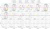 |
Fig. 1. (u, v) coverage for all sources observed during the EHT 2017 campaign, as summarized in Table 1, combining all available visibility detections for all days and bands, averaged in 120 s intervals. The two circles in each panel correspond to the fringe spacing characterizing an instrumental resolution of 25 and 50 μas. JCMT-SMA and ALMA-APEX are the very short intrasite baselines, shown as black data points near the origin of the (u, v) coordinate system (when available). JCMT and SMA are shown as “Hawai’i”, while ALMA and APEX are shown as “Chile”. |
Summary of the EHT 2017 observations at 230 GHz.
With this work, we inaugurate a 230 GHz catalog of sources that will grow with subsequent EHT campaigns. In particular, this work adds 230 GHz observations to the large existing sample of sources from surveys at lower frequencies. Since the mid 1990s, 86 GHz surveys have been carried out, first with the Coordinate Millimeter VLBI Array (CMVA; Rogers et al. 1995; Beasley et al. 1997; Rantakyro et al. 1998; Lonsdale et al. 1998; Lobanov et al. 2000; Lee et al. 2008), which was ultimately succeeded by the Global Millimeter VLBI Array (GMVA; Lee et al. 2008; Nair et al. 2019). Pushkarev & Kovalev (2012) carried out a survey at 2 GHz and 8 GHz using a combination of the Very Long Baseline Array (VLBA) and up to ten geodetic antennas. The long-running MOJAVE1 (Kellermann et al. 2004; Lister & Homan 2005; Kovalev et al. 2005; Homan et al. 2006; Cohen et al. 2007; Lister et al. 2009, 2018, 2021) and VLBA-BU-BLAZAR/BEAM-ME2 programs (Jorstad et al. 2017; Weaver et al. 2022) supply data at intermediate frequencies 15 GHz and 43 GHz, respectively, observed with the VLBA. Surveys at 5 GHz have been carried out with the VLBA in the frame of the VLBA imaging and polarimetry survey (VIPS; Helmboldt et al. 2007, 2008) and the VLBI space observatory program (VSOP; e.g., Dodson et al. 2008).
Characteristic properties of AGN jets may be revealed using a statistical approach to the investigation of the brightness temperature and its dependence on frequency, and in turn, on the distance from the central engine (Blandford & Königl 1979). Given a sufficiently large sample size, such an approach remains robust against uncertainties related to properties of individual sources, such as poorly constrained inclination and bulk flow velocity, as long as errors are uncorrelated. Adding measurements at higher frequencies is expected to greatly enhance the results of such statistical analyses, extending the investigated jet region closer to the SMBH and thus allowing for more accurate tests of the inner jet models, including their launching (e.g., Blandford & Znajek 1977; Blandford & Payne 1982) and acceleration in the vicinity of the true central AGN engine (e.g., Blandford & Königl 1979; Marscher 1995; Heinz & Begelman 2000; Vlahakis & Königl 2004). Throughout this paper we adopt a cosmology with H0 = 67.7 km s−1 Mpc−1, Ωm = 0.307, and ΩΛ = 0.693 (Planck Collaboration XIII 2016).
2. EHT results
2.1. EHT observations and data reduction
Eight facilities participated in the EHT observing campaign on April 5-11, 2017: The Atacama Large Millimeter/submillimeter Array (ALMA, A, operating as a phased array; Matthews et al. 2018; Goddi et al. 2019) and the Atacama Pathfinder Experiment (APEX, X) telescopes in Chile; the Large Millimeter Telescope Alfonso Serrano (LMT, L) in Mexico; the IRAM 30 m telescope (PV, P) in Spain; the Submillimeter Telescope (SMT, Z) in Arizona; the James Clerk Maxwell Telescope (JCMT, J) and the Submillimeter Array (SMA, S) in Hawai’i; and the South Pole Telescope (SPT, Y) in Antarctica. Two frequency bands, each 2 GHz wide, centered at 227.1 GHz (LO band) and 229.1 GHz (HI band) were recorded. For a detailed description of the EHT array instrumental configuration see The Event Horizon Telescope Collaboration (2019b).
Following correlation, the data were reduced using the EHT-HOPS (Blackburn et al. 2019) and rPICARD (Janssen et al. 2019) pipelines to independently validate the results (The Event Horizon Telescope Collaboration 2019c). The EHT calibration procedures are described in detail in The Event Horizon Telescope Collaboration (2022b), with minor updates with respect to The Event Horizon Telescope Collaboration (2019c). Whenever applicable, polarization leakage was calibrated following The Event Horizon Telescope Collaboration (2021a) and Issaoun et al. (2022). The electric vector position angle (EVPA) calibration requires persistent participation of ALMA in the EHT observing array. As a consequence, the polarization leakage calibration could only be applied in a straightforward way to sources with coverage as good or better than that of 3C 273 (see Table 1 and Fig. 1, as well as Paraschos et al. 2024 for further details). In particular, the seven sources introduced in this paper (Table 1) were not calibrated for polarization leakage and the absolute EVPA. This issue has minimal impact on the total intensity analysis, but the polarimetric analysis is affected, see Appendix A. While EHT resolves structures on ∼10–500 μas angular scales, simultaneous ALMA-only measurements of flux densities and fractional polarization at 212–230 GHz at angular resolutions of ∼ 1 arcsec have been reported for a number of observed sources by Goddi et al. (2021), constraining the total flux density of the core and the compact jet.
2.2. EHT data sets and model fitting
A summary of the EHT observations in April 2017 is given in Table 1. The “Volume” column contains the number of scan-averaged detected visibilities (that is, time-averaged for several minutes, depending on a particular schedule, with separate polarimetric correlation products counted individually), indicating the relative constraining power of the respective data sets; see also Fig. 1 for a comparison of the (u, v) coverage between the different EHT data sets. For Cygnus X–3 we only measured a short (intrasite) baseline flux density, preventing us from estimating source compactness. Apart from the two galactic sources (Sgr A* and Cyg X–3), the EHT data set contains observations of sixteen AGN sources, which are the subject of the analysis presented in this paper. For these sources we provide estimates of the black hole masses and Doppler factors in Appendix B.
Whenever a dedicated study of an individual EHT target is available (“Ref.” column in Table 1), we used source parameters reported therein. For the remaining seven AGN sources with very sparse (u, v) coverage and with no dedicated analysis published, we performed geometric model fitting with linearly polarized circular Gaussian components using eht-imaging (Chael et al. 2016, 2022; Roelofs et al. 2023), exploiting heuristic optimization tools implemented in SciPy (Virtanen et al. 2020) to search for the best-fit solution. For each of these sources we used all available data (LO and HI bands, all available days) to constrain a single geometric model. The number of polarized circular Gaussian components was chosen based on the minimal number of the model degrees of freedom required to obtain a high quality fit to visibility amplitudes, closure phases, and fractional linear polarizations, generally characterized by the reduced χ-square χn2 < 2.
For five out of seven sources (1749+096, 1055+018, BL Lac, J0132–1654, J0006–0623) we modeled the morphology with two or three circular Gaussians, presented in Fig. 2. Low visibility amplitudes around ∼1 Gλ for 1055+018 were identified as LMT miscalibration related to pointing issues (see also The Event Horizon Telescope Collaboration 2019c for a summary of issues with LMT in 2017). These points were downweighted for the amplitude fitting, but preserved for the closure phase fitting. For the other two out of seven sources (CTA 102 and 3C 454.3), a single circular Gaussian was sufficient to interpret the observations. We assume that the core components are nearly circularly symmetric.
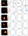 |
Fig. 2. Models of the EHT sources obtained through (polarized) circular Gaussian model fitting with at least two components. Blue crosses in the left column indicate positions of individual components. Contours represent 0.1, 0.3, 0.5, 0.7 and 0.9 of the peak total intensity. EHT observing beams are shown with dashed-line ellipses, to give a sense of the diffraction limited resolution supported by the data sets. We show consistency between models (black) and data (blue) for visibility amplitudes, closure phases, and absolute values of fractional visibility polarization. Closure phases are shown as a function of combined baseline length, which corresponds to a quadrature sum of lengths of all baselines from a given triangle. The visibility domain fractional polarization may exceed unity for resolved sources, such as is the case for 1749+096. The data shown contain detections only and no upper limits. |
In the cases of BL Lac (Casadio et al. 2021), 1055+018 (Weaver et al. 2022) and several other sources, the 230 GHz model fit structure is consistent with images obtained at lower frequencies. For other sources, the separation of scales between the highest angular resolution images available so far and our modeling results makes such a comparison difficult. In particular, we identify an east-west structure in 1749+096, well constrained by the data, but perpendicular to the jet observed at lower frequencies, extending in the north direction (Weaver et al. 2022). While in this paper we focus on the total intensity properties of the sources, we also obtained linear polarization results for the Gaussian components, reported in Appendix A (Fig. A.1) along with detailed parameters of the fitted Gaussian models (Table A.1) and more technical comments regarding the model fitting procedures.
The EHT measurements of the 230 GHz VLBI cores, discussed further in this work, can be represented on a plane of core brightness temperature (see Sect. 3.3) against isotropic spectral core luminosity Lν ∝ SνDL2 for the luminosity distance DL, see Fig. 3. This representation emphasizes the differences between the types of observed sources within the inhomogeneous EHT data set, with radio galaxies at the lower luminosity and brightness temperature corner of the figure, and luminous, high brightness temperature quasars in the opposite corner. The figure does not show Sgr A*, with 230 GHz spectral luminosity Lv ∼ 1023 erg s−1 Hz−1, over five orders of magnitude below the least luminous AGN in the sample.
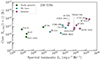 |
Fig. 3. Core brightness temperature against core synchrotron spectral luminosity for the EHT 2017 sample of 16 AGN sources. The sources cluster into categories of radio galaxies, BL Lacs (blazars), and quasars. |
3. Measurements in the EHT+ data set
We consider sixteen AGN sources observed by the EHT, as summarized in Tables 1 and 2. For this set of sources, we additionally use measurements obtained at lower frequencies. We refer to this collection of measurements as the EHT+ data set. The EHT+ data set below 230 GHz spans a range of frequencies from 2 to 86 GHz, taken from a variety of surveys and monitoring efforts. At 1.66, 4.84, and 22.24 GHz we used measurements from the RadioAstron space VLBI program (Kardashev et al. 2013; Kovalev et al. 2020; Kovalev et al., in prep.), comparing them to VLBA data at 2.3 GHz (single-epoch, Pushkarev & Kovalev 2012) and 24 GHz (multiepoch, de Witt et al. 2023), as well as measurements from the VSOP program at 5 GHz (Dodson et al. 2008). Further VLBA data include 8 GHz (Pushkarev & Kovalev 2012), 15 GHz (MOJAVE, Homan et al. 2021), and 43 GHz (VLBA-BU-BLAZAR, Weaver et al. 2022). At 86 GHz, we used results obtained in a single-epoch GMVA AGN survey (Lee et al. 2008). In addition to these survey results, we used core brightness temperature measurements for M 87 at 43 GHz (Cheng et al. 2020) and Centaurus A at 8.4 and 22.3 GHz (TANAMI3, Müller et al. 2011). In order to increase the homogeneity of the data set and limit the impact of low resolution bias we exclude measurements obtained with arrays lacking long baselines, such as those procured using the Korean VLBI Network (KVN) for frequencies of 23, 43, 86, and 129 GHz (Lee et al. 2016b).
3.1. multifrequency power law fits
We aim to characterize the dependence of the measured quantities (VLBI core size, flux density, brightness temperature) on the frequency with a power law model. However, individual properties of sources differ, scaling the observables. These include their cosmological redshift, Doppler factor, intrinsic source power and distance, as well as their intrinsic variability. Hence, the scaling parameter b in a power law bνa is generally source-specific and the inhomogeneous data set may not be self-consistently fitted with a single power law. Thus, in this paper we treated the scaling b as a source-specific nuisance parameter and characterized the slope a for the EHT+ data set by studying 16 individual sources and subsequently aggregating the results. The parameter b absorbs effects impacting the observables for the individual sources as a constant (frequency-independent) factor, such as cosmological redshift, constant Doppler factor, or intrinsic power. It preserves the relative impact of effects depending on the frequency or location along the jet such as acceleration and energy conversion, which we studied here.
To evaluate the characteristic power law slope in a frequency dependence of a given quantity for the entire EHT+ sample, we considered a set of N = 16 slopes ai, fitted separately for individual sources. We extracted their mean value m and standard deviation σ, and used  as our estimate of the characteristic power law slope in the population. In Appendix B we further discussed this choice and compare it with alternative approaches, such as directly fitting all measurements with a single power law, demonstrating robustness of the estimated slopes.
3.2. Core size and flux density
We estimated the VLBI core diameter θ and flux density Sν using geometric Gaussian model fitting (see Sect. 2.2), identifying the core with the brightest of the fitted Gaussian components, that is, the component with the largest measured brightness temperature value. Both core size and core flux density parameters are generally subject to significant systematic uncertainties, related to the sparse (u, v) coverage. An interferometer is a spatial filter and the correlated flux density measured on the long baselines misses the resolved-out emission from structures larger than ∼λ/BL, where BL is the baseline length. This effect should not negatively affect the characterization of the compact cores with the EHT, but may be relevant for extremely long baselines and lower observing frequencies, as is the case for the RadioAstron observations. Table 2 compares 230 GHz flux densities measured by the connected ALMA array (∼100–300 kλ), the JCMT-SMA (J-S) baseline (∼100 kλ), as well as the ALMA-APEX (A-X) baseline (∼1.5 Mλ). There are indications of losses in VLBI flux density measurements in comparison with connected-element ALMA interferometry for comparable baseline lengths (see Appendix C). For the EHT data sets, ALMA flux densities can generally be considered to be the most reliable; thus, when available, they were used to calibrate the short VLBI baselines. This is the case in Table 2, where we give VLBI measurements for short intrasite baselines without scaling them to ALMA measurements, but the compact VLBI and core flux densities follow subsequent rescaling for sources with sufficient ALMA-only data (network calibration; Blackburn et al. 2019). Nonetheless, the additional flux density uncertainty of ∼20% related to the ALMA-VLBI discrepancy (Appendix C) is subdominant with respect to other systematics and does not significantly impact our results.
Flux densities, core sizes, and core brightness temperatures at 230 GHz measured during the 2017 EHT observing campaign.
In contrast to the flux density, the estimate of the core size may indeed be affected by the limited instrumental resolution. The configuration of the 2017 EHT array yields extreme angular resolution, but suffers from generally sparse coverage and lack of baselines probing milliarcsecond scales. Therefore, the dynamic range of the reconstructions is often low, and extended components are resolved out. Hence, studying jets on milliarcsecond and larger angular scales with the 2017 EHT array is effectively impossible. The array is, however, well suited for studying dominant, bright and compact core components in AGN systems. Indeed, none of the considered data sets shows clear indication of compact unresolved structures, though some of the lower frequency measurements in the EHT+ data set do – in those cases the core size estimates correspond to resolution-dependent upper limits.
The 15, 22, and 43 GHz measurements used in this analysis were respectively obtained from year- or decade-long surveys as parts of the MOJAVE program, the K-band celestial reference frame survey, and the VLBA-BU-BLAZAR/BEAM-ME programs. At higher frequencies, such monitoring programs are not available; 86 and 230 GHz measurements were collected in single-snapshot surveys. They may therefore not properly reflect the usual behavior of the individual variable sources. As an example, fluctuations of the 230 GHz compact ring-like core of M87 between 0.5 and 1.0 Jy were reported by Wielgus et al. (2020). The intrinsic source variability potentially contributes to uncertainty, if, for instance, a source happened to be in a flaring state during the observation. In the case of RadioAstron data, the correlation between increased source activity and availability of detections was addressed by treating the obtained brightness temperatures as upper limits.
Figure 4 shows the flux density and size of the VLBI cores in the EHT+ data set, as well as the resulting brightness temperatures, against frequency measured in the host frame of the AGN (corrected for the cosmological redshift, hereafter referred to simply as “host frame”). For 2, 5, and 22 GHz there are two sets of points, high angular resolution RadioAstron (semi-transparent markers) and lower resolution observations (solid-color markers). The systematic difference in the estimated core size is evident, with RadioAstron finding cores about an order of magnitude more compact. As a consequence, brightness temperatures inferred from RadioAstron observations sometimes approach 1014 K, which is difficult to reconcile with the assumption of incoherent synchrotron emission from relativistic electrons as it would require untypically high Doppler boosting (Kovalev et al. 2016). Another effect possibly limiting the accuracy of the obtained measurements, particularly at lower frequencies, is related to blending between the core and the foreground jet components.
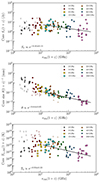 |
Fig. 4. Measurements of the core flux density (top), size (middle), and brightness temperature (bottom) obtained using the EHT+ data set of AGN sources, as a function of frequency in the host frame. The 15–230 GHz ground array data in each panel are approximated by power law fits (solid lines, obtained as detailed in Sect. 3.1) and the fit results are annotated. The faded data points are the RadioAstron measurements, while regular data points at the same frequencies correspond to VLBA and VSOP measurements; for comparability, we color the 1.66 GHz (L band) RadioAstron points the same as the 2 GHz (S band) VLBA points. The slope of the core flux density is shallow, Sν ∝ ν−0.4. The core size decreases with frequency (and, in turn, increases with the distance from the central engine) as θ ∝ ν−0.6; the brightness temperature decreases with frequency as Tb ∝ ν−1.0. |
In Fig. 4 we also present power law fits to ground array data from 15–230 GHz, that is, excluding the lower frequency measurements suffering from the aforementioned systematic shortcomings. The calculation of the power law slope follows the methodology described in Sect. 3.1. The spectra are almost flat (top panel), at most slightly decreasing with frequency as Sν ∼ ν−0.4 for 15 GHz and above, as expected from VLBI cores at high observing frequencies. The estimated core size decreases as θ ∼ ν−0.6 in the range of 15–230 GHz. This decrease is less steep than the expected dependence dominated by the instrumental resolution effects ∼ν−1. The core size vs frequency panel of Fig. 4 indicates steepening of the slope at 2–8 GHz, in the region possibly more affected by the limited resolution and potentially also by scatter-broadening. This further justifies only selecting 15–230 GHz measurements for the power law fitting.
3.3. Brightness temperature
The brightness temperature Tb is an important tool to probe the nature and launching mechanisms of astrophysical jets. In the emitter frame, the intrinsic brightness temperature Tb, int equals the equivalent black body temperature given the source surface brightness. It serves as a proxy of the temperature of electrons emitting the observed synchrotron radiation, enabling the characterization of the energy partition between plasma and the magnetic field, parametrized with the ratio of emitting particles energy to magnetic energy η assuming self-absorbed synchrotron radiation (Readhead 1994; Homan et al. 2006).
The observed Tb, obs differs from the intrinsic value by a cosmological factor (1 + z)−1 (usually known well) and the Doppler factor δ depending on the bulk outflow velocity and the jet viewing angle (usually known poorly),
 (1)
(1)
where Tb, eq ≈ 5 × 10¹⁰ K is the equipartition brightness temperature (Readhead 1994). Following Eq. (1), in this work we denote the cosmological redshift-corrected brightness temperature (that is, measured in the frame of the host galaxy) simply with Tb ≡ Tb, obs(1 + z) = δTb, int. For a circular Gaussian source model the peak brightness temperature in Kelvins can be calculated as
 (2)
(2)
where Sν is the measured correlated flux density at the observing frequency ν, and θ is the angular size of the source, defined as the full width at half maximum (FWHM) of the fitted Gaussian. By using a simple Gaussian model, we neglect the transverse structure of the jet. The frequency in the host frame is larger than the one observed by a factor (1 + z), but in the comoving frame of the emitting plasma it is reduced by a factor of δ, typically exceeding unity for jet sources.
Since modeling the source structure using sparse VLBI data is subject to large systematic uncertainties, model-agnostic estimates based solely on visibility measurements provide potentially useful limits on the brightness temperature (Lobanov 2015):
 (3)
(3)
 (4)
(4)
with maximum baseline length BL, corresponding visibility amplitude Vq and its uncertainty σq. The values of BL are reported in Table 1; core component flux density, size, and peak brightness temperature of the source model Tb, obs(1 + z), as well as the visibility-only brightness temperature estimates can be found in Table 2. The latter indicate broad consistency with the brightness temperatures obtained based on Gaussian component modeling.
In the case of sources with relatively good (u, v) coverage, with detailed analyses described in dedicated papers (e.g., Janssen et al. 2021; Gomez et al., in prep.), we report core parameters following the imaging results presented therein, without resorting to approximated geometric modeling with Gaussian components.
The resulting measurements of brightness temperature Tb are shown in the bottom panel of Fig. 4. The systematic difference between measurements with long RadioAstron baselines (semi-transparent markers at 2, 5, and 22 GHz) and the other observations at the same frequencies obtained with the VLBA and as part of the VSOP program are clearly visible. A power law fit to the data at frequencies of 15 GHz and larger indicates a slope with an index of −0.95 ± 0.13, fitted with the methodology described in Sect. 3.1; see also the discussion in Appendix B.
4. Modeled quantities
4.1. Distance from the VLBI core to the black hole
We adopt the framework for relativistic jets established by Blandford & Königl (1979) and Königl (1981), assuming a supersonic, conical jet with an opening angle ϕo, and a viewing angle ι. We refer to this setup as the BK model. The jet bulk Lorentz factor γj is constant in this framework, and the jet magnetic field B ∝ r−m and particle density N ∝ r−n are described as functions of the distance r from the jet origin.
Following Lee et al. (2016a), we employ a measure for the distance of the observed VLBI core to the true central engine under the assumption of equipartition between the particles in the jet and the magnetic field. The VLBI core is defined as the region where the optical depth reaches unity. Then, the physical distance (measured along the jet) of the VLBI core to the true central engine is (Lobanov 1998):
![Mathematical equation: $$ \begin{aligned} r = \left( \frac{B_1^{k_{\rm b}}}{\nu (1+z)}\left[6.2\times 10^{18} C_2(\alpha ) \delta ^\epsilon \phi _{\rm o} N_1\right]^{1/(\epsilon +1)}\right)^{1/k_{\rm r}} \mathrm{pc}, \end{aligned} $$](/articles/aa/full_html/2025/03/aa52600-24/aa52600-24-eq6.gif) (5)
(5)
where B1and N1 are, respectively, the magnetic field strength and electron number density at r1 = 1 pc distance from the jet origin, δ is the jet Doppler factor δ = (1 − β cos ι)−1γ−1, C2(−0.5) = 8.4 × 10¹⁰ cgs (Pacholczyk 1970; Königl 1981) and
![Mathematical equation: $$ \begin{aligned} k_{\rm r}&= \left[(3-2\alpha )m+2n-2\right]/(5-2\alpha ), \end{aligned} $$](/articles/aa/full_html/2025/03/aa52600-24/aa52600-24-eq7.gif) (6)
(6)
 (7)
(7)
 (8)
(8)
In this work we do not attempt to use Lorentz factors, Doppler factors, and viewing angles measured for individual sources. Instead, following previous analyses, we assume a characteristic bulk Lorentz factor γj = 10 for the entire sample and N1 = 5 × 103 cm−3 at a distance of r1 = 1 pc from the black hole (Lee et al. 2016a). For the intrinsic and observed opening angles, we set ϕ = 0.01 rad ≈ 0.6° and ϕo = ϕcscι with the viewing angle ι = 0.1 rad, resulting in δ ≈ 10. Furthermore, following Königl (1981) and Lobanov (1998) we assume energy equipartition and adopt m = 1, n = 2, kr = 1, kb = 2/3, and ϵ = 2, with α = −0.5 (Sν ∝ να). The magnetic field strength B1 at 1 pc can be expressed through the total synchrotron luminosity Lsyn, following Blandford & Königl (1979):
 (9)
(9)
where DL is the luminosity distance to the source and Sint is the integrated, redshift corrected observed synchrotron flux density, integrated in the host frame frequency range between 1 GHz and 700 GHz by fitting a power law in ν to measured Sν of each individual object. Equation (5) then takes a form
 (10)
(10)
with a constant K incorporating the assumed BK model parameters. In order to correct Lsyn for the Doppler effect, the right hand side of the Eq. (10) would be scaled by ∼δ−1, where the exact power depend on detailed physical assumptions (Ghisellini et al. 1993). The other Doppler factor present in Eq. (5) was absorbed into the K factor in Eq. (10) and for the assumed parameters corresponds to δ2/3, so the overall dependence of the radius estimate on the Doppler factor is shallow δ−1/3. In previous studies, the model described above was applied to measurements made at frequencies up to 86 GHz (Lee et al. 2016a; Nair et al. 2019).
The choice of particular fixed BK model jet parameters for an inhomogeneous sample of sources such as EHT+ is justified by the fact that the sample is dominated by quasars and BL Lac objects. Furthermore, we are mostly interested in the power law dependence. Essentially, with the methodology described in Sect. 3.1, the only BK model information impacting the power law index fits shown in Fig. 5 is that r ∼ ν−1/kr. We comment further on the impact of source-specific corrections in Appendix B, where we incorporate Doppler factor corrections following estimates given in Table B.2.
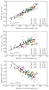 |
Fig. 5. Core size (top), brightness temperature (middle), and magnetic field estimate (bottom) obtained from the EHT+ data set as a function of the distance to the central engine. The 15–230 GHz data in each panel are approximated by power law fits (solid lines, obtained as detailed in Sect. 3.1) and the fit results are annotated. The faded data points at are the RadioAstron measurements, while the filled markers correspond to VLBA observations. For comparability, we color the 1.66 GHz (L band) RadioAstron points the same as the 2 GHz (S band) VLBA points. For a M• = 108 M⊙ black hole 1 pc =2 × 10⁵rg with gravitational radius rg = GM•/c2. |
4.2. Magnetic field strength
The magnetic field strength of a synchrotron self-absorbed core can be roughly estimated as (e.g., Section 5.3 ofCondon & Ransom 2016)
 (11)
(11)
where we do not attempt to correct for the Doppler factor, which would increase B in the emitter’s frame by a factor δ. While this estimate is independent of the BK jet model assumptions, it incorporates a very simplistic model for the emission spectrum. We found that Eq. (11), while having the same functional dependence of  , results in a magnetic field ∼25 times stronger compared to the BSSA estimator of Marscher (1983) for identical input; the latter, however, is only applicable at the synchrotron turnover frequency. Hence, we expect a systematic upward bias of B. Nonetheless, the relative differences and the slopes remain useful for interpretation, provided that the VLBI cores do not become optically thin at the higher observing frequencies.
5. Results and discussion
The observations collected in the EHT+ data set are presented in Fig. 4. In the framework of the BK jet model, we expect the intrinsic brightness temperature Tb, int to not exceed the equipartition limit Tb, eq ≤ 1011 K (Readhead 1994; Lähteenmäki et al. 1999; Singal 2009) and, more fundamentally, the inverse Compton limit Tb, IC ∼ 5 × 10¹¹ K (Kellermann & Pauliny-Toth 1969; Nair et al. 2019). Observed brightness temperatures in excess of these limits may be caused by large Doppler factors as Tb, obs(1 + z) = δeqTb, eq. The equipartition Doppler factors necessary to fulfill this condition are δeq < 10 in the EHT sample at 230 GHz. Hence, from measured values of Tb alone, all sources are consistent with the equipartition limit without invoking unreasonably high Doppler factors at high observational frequencies. When interpreting brightness temperature measurements, we additionally make the crucial assumption that we observe self-absorbed, optically thick cores, and that they do not become fully optically thin at high observing frequencies.
In some cases, we observed 230 GHz brightness temperatures significantly below Tb, eq, which are better explained by a magnetically dominated inner jet, in which case the observed brightness temperature is reduced by η2/17 < 1, following Eq. (1). On the other hand, very large brightness temperatures obtained by RadioAstron at 1.7 and 5 GHz, reaching 1014 K, are difficult to reconcile with the assumption of equipartition, requiring unrealistically large equipartition Doppler factors. Instead, a more complicated core geometry or scattering sub-structure may play a role in driving up the brightness temperature (e.g., Johnson & Gwinn 2015; Johnson et al. 2016). The RadioAstron measurements were excluded from the power law fitting, which was limited to 15–230 GHz ground array data.
5.1. Tweaking the Blandford-Königl model parameters
The new observations at 230 GHz confirm that the brightness temperature Tb increases with the distance from the central engine, that is, it becomes larger for lower observing frequencies. Indications of such a trend were previously found by Lee et al. (2008) and Nair (2019). While quantifying these trends is hindered by significant systematic uncertainties, in Sect. 3 we reported the core size and brightness temperature dependence on the observing frequency θ ∝ ν−0.6 and Tb ∝ ν−1.0.
To estimate the radial distance from the black hole to the VLBI core, we set up a jet model using various assumptions, as described in Sect. 4. For a conical BK jet, the core diameter scales with frequency as θ ∝ r ∝ ν−1/kr, where kr = 1 in the case of equipartition. This immediate tension with the θ ∝ ν−0.6 dependence observed in Fig. 4 could be alleviated by a larger value of kr. Following Eq. (6), kr depends on the assumed radial density and magnetic field strength profiles; a larger kr corresponds to a faster decay of these quantities with radius. In our example, changing B ∝ r−1 to B ∝ r−2 would be enough to reconcile the conical BK model with the observed relationship between core size and frequency. A steep decrease of the modeled magnetic field strength with radius is also found under the BK assumptions, see the bottom panel of Fig. 5 and Sect. 5.3.
Alternatively, the mismatch between our measurements and the brightness temperature, jet diameter and magnetic field strength radial dependence predicted by the BK model may be due to a transition from a parabolic to a conical jet geometry. There is ample observational evidence for a parabolic geometry of the jet base (e.g., Asada & Nakamura 2012; Hada et al. 2016, 2018; Okino et al. 2022; Ricci et al. 2022). Calculating the distances to the central engine using the BK model (Sect. 4 and Fig. 5), we find θ ∝ r0.7, which deviates from the expectations for a conical jet (θ ∝ r1.0) in the direction of a more parabolic structure (θ ∝ r0.5). However, this predominantly shows the inconsistency of the canonical BK model with the data.
The brightness temperature is a derivative quantity of measured core size and flux density, Tb ∝ Sνν−2θ−2. For the canonical BK jet, Sν is flat and θ ∝ ν−1, resulting in a flat Tb. From the EHT+ measurements we found a mildly negative slope of Sν, and the slope of θ(ν) is shallower than the BK prediction, adding up to the observed Tb ∝ ν−1.0 dependence. While adjusting kr, as discussed above, would take care of the impact of the core size trend on Tb, it would not address the impact of the flux density trend.
5.2. Doppler factor evolution and energy conversion
Alternatively, the assumptions of a constant jet velocity or energy partition factor may need to be abandoned, as Tb ∝ δη2/17. With the power law slopes found in the bottom panel of Fig. 4 we obtain
 (12)
(12)
where νint = νobs(1 + z)/δ is the frequency in the emitter’s frame. If we assume η = const., we find a constant intrinsic brightness temperature for a physically reasonable  for kr = 1. Hence, the Doppler factor grows more rapidly in the region close to the black hole. Allowing for η to increase with radius, as magnetic energy is transferred to particles, adds another degree of freedom and will generally decrease the slope of δ(r). If we additionally require a flat spectrum measured in the jet frame, given the observed Sν slope (top panel of Fig. 4), we arrive at δ ∝ r−0.3 and η ∝ r−3.1. These findings are a direct consequence of the observations and are independent of the BK model assumptions other than the choice of kr with ν ∝ r−kr.
The growth of the Doppler factor with radius is a well motivated conclusion in the context of compact-scale AGN jets, since the bulk acceleration of the outflow must take place somewhere between the black hole and the parsec scales. A model in which both δ and η grow with radial distance from the black hole is consistent with a magnetically accelerated jet (Vlahakis & Königl 2004), transitioning from the magnetically (or Poynting) dominated innermost region to energy equipartition (or dominance of particle kinetic energy) further away. A different physical scenario has been proposed by Melia & Konigl (1989) and Marscher (1995), where an electron-positron jet is accelerated to ultra-relativistic energies at compact scales and subsequently decelerated through inverse-Compton scattering with external photons. In the process, high-energy emission in X-ray and γ-ray bands is produced, and the jet becomes progressively brighter in radio band further away from the black hole. This scenario was discussed in the context of the brightness temperature statistics by Lee (2014). We consider this model to be less physically plausible (see, e.g., Sikora et al. 1996, on the role of radiation drag for jet deceleration).
Another caveat is the possible impact of a change in viewing angle ι in a bending jet on the radial profile of the Doppler factor δ. Observations confirm the curved structure of some of the compact-scale jets in this work (e.g., Issaoun et al. 2022; Jorstad et al. 2023), further increasing the spread of brightness temperatures measured in the EHT+ sample with the viewing angle varying between the observing frequencies. If a certain source was bright at low frequencies due to a favorable viewing angle, it would show a lower core Tb than expected at higher frequencies, given a bend away from the favorable inclination in the more inner part of the jet. Moreover, an acceleration to speeds above β = v/c = cos ι (or γ > cscι) would decrease the observed Tb again, as the radiation becomes increasingly beamed along the jet axis, away from the observer at inclination ι. At large angular scales, we expect jets to be better described by the BK model, with a flat core spectrum Sν(ν), a continued high frequency trend in θ(ν), and a flattening of Tb(ν). This seems to be the case for the 2 and 5 GHz observations shown in Fig. 4, although the conclusions are uncertain given the large spread and the small size of the sample.
5.3. Magnetic fields
The bottom panel of Fig. 5 shows the magnetic field estimates against the distance to the black hole, calculated with the BK model. For a canonical BK model (i.e., flat Tb), as described in Sect. 4, Eq. (11) gives B ∝ ν ∝ r−kr, self-consistent assuming m = kr = 1. However, since we measure Tb ∝ ν−1, Eq. (11) gives B ∝ ν3 ∝ r−3kr, consistent with the result from fitting the data points in the bottom panel of Fig. 5. However, 3kr = m would imply m + n = 1, requiring very shallow dependence of gas density and magnetic field strength with radius. These observations are thus in tension with the BK model. Correcting for the Doppler factor in Eqs. (10) and (11) would allow the steepness of the radial dependence of B to be mitigated.
Magnetic field estimates for the most compact scales reach B ∼ 103 G, which is consistent with some predictions for magnetized accretion disks (Field & Rogers 1993). In the special case of M 87, where the central engine can be resolved, a correction for the over-estimation of the magnetic field (see Sect. 4.2) would bring down the obtained field strength to a value comparable to estimates made by the EHT in the previous studies (The Event Horizon Telescope Collaboration 2021b). Across the EHT+ sample the field strength decreases by about seven orders of magnitude toward the largest probed scales of ∼106rg (∼10 pc). At distances larger than one parsec estimated fields of B ∼ 10−4 G become comparable to the μG-field of the ambient medium (McKee & Ostriker 2007; Beck 2015). In the BK jet framework, the magnetic field components perpendicular and parallel to the jet axis behave as B⊥ ∝ r−1 (Blandford & Königl 1979) and B∥ ∝ r−2 (Königl 1981), respectively. We find that the B(r) slope is steeper than −1, consistent with the steeper B(r) slope inferred from the observed core size dependence on frequency. This supports the presence of poloidal (jet-parallel) magnetic fields in the inner jet regions, possibly forming a mixed helical geometry (Gabuzda et al. 2017). A steep decrease of the magnetic field strength with radius may also be indicative of an efficient conversion of magnetic energy into kinetic energy of particles through, for example, magnetic reconnection. The estimated slopes for some of the sources inspected individually are steeper than −3, following the decrease of the observed brightness temperature with frequency. This may be a consequence of rapid acceleration and a related radial increase of Doppler factor, unaccounted for in the BK model. Given the dependencies of B∥ and B⊥, a shallower slope in between −2 and −1 could be interpreted as a helical, but coherent field; the steep measured slope could hence indicate a loss of magnetic field coherence or strong dissipation through magnetic reconnection at larger distances. A steep slope of B(r) could also indicate a decrease of the optical depth at high observing frequencies, biasing the magnetic field estimates upward in the more compact regions.
6. Summary and conclusions
In this work, we presented an analysis of the full EHT 2017 observational data set: the first 230 GHz VLBI campaign of this magnitude. We compiled the EHT+ sample of sixteen AGN sources observed by the EHT, along with their VLBI observations available at lower frequencies (2–86 GHz). For seven of these AGN sources we presented visibility domain modeling of the EHT data; the analyses of the remaining nine sources were given in separate papers. We first studied the change of the VLBI core flux density, size, and brightness temperature as a function of frequency in the EHT+ data set. Despite large scatter in the measurements, related to individual source properties, the joint analysis reveals a shallow dependence of the core size on frequency θ ∝ ν−0.6 and a systematic decrease of the brightness temperature with frequency Tb ∝ ν−1.0, indicating an increase of brightness temperature with the distance from the AGN central engine. These findings are qualitatively consistent with previous studies using lower and fewer observing frequencies.
We demonstrated that properties of AGN jet sources constrained by the VLBI observations at 15–230 GHz are incompatible with the standard BK model of a conical jet with constant Lorentz factor and energy partition. Discussing the impact of variations of the BK model parameters and the jet collimation profile led us to the conclusion that either a bulk acceleration of the jet (an increase of the Doppler factor with the jet radius), or a transfer of energy from the magnetic field to the emitting particles is required to interpret the data.
Both effects may occur simultaneously, and both are expected to play a role in compact scale jets based on theoretical models. A radial dependence of the Doppler factor δ ∝ r0.5(or a slightly shallower one, in the case of a radially evolving energy partition), could explain the observations. Our findings are consistent with these effects occurring gradually across the innermost parsec of the jet, or within ∼105 rg from the central black hole, with most of the Doppler factor increase occurring very close to the central engine.
Additionally, using the BK model, we estimated a steep decrease of magnetic field with radius B ∝ r−3, which is in tension with the underlying assumptions. The steepness of the slope may be reduced by incorporating a radially increasing Doppler factor, once again hinting at bulk acceleration of the jet. Alternatively, a strong dissipation of the magnetic energy may be taking place in the compact region of the AGN jets.
Subsequent EHT campaigns will deliver 230 GHz VLBI measurements for a larger number of objects, increasing our EHT+ sample size and thus its statistical robustness. With more high quality data it will become feasible to apply (possibly frequency dependent) Doppler corrections to individual sources. Further, studying jet kinematics on EHT scales through tracking of individual moving features and comparing these results with lower frequency VLBI data could conclusively demonstrate the radial profile of jet acceleration, breaking degeneracies in our theoretical models. Finally, an extension of VLBI capabilities to 345 GHz, which is already in the process of being implemented within the EHT, will provide insight on AGN jets on even more compact scales.
Data availability
A table compiling measured VLBI core flux densities, FWHM sizes and brightness temperatures, as well as the derived distances to the black hole, magnetic field strengths and synchrotron luminosities is available in electronic form at the CDS via anonymous ftp to cdsarc.cds.unistra.fr (130.79.128.5) or via https://cdsarc.cds.unistra.fr/viz-bin/cat/J/A+A/695/A233.
Monitoring of jets in active galactic nuclei with VLBA experiments.
Blazars entering the astrophysical multimessenger era.
Tracking active galactic nuclei with Austral milliarcsecond interferometry.
References
- Agudo, I., Thum, C., Gómez, J. L., & Wiesemeyer, H. 2014, A&A, 566, A59 [NASA ADS] [CrossRef] [EDP Sciences] [Google Scholar]
- Asada, K., & Nakamura, M. 2012, ApJ, 745, L28 [NASA ADS] [CrossRef] [Google Scholar]
- Baczko, A.-K., Kadler, M., Ros, E., et al. 2024, A&A, 692, A205 [NASA ADS] [CrossRef] [EDP Sciences] [Google Scholar]
- Beasley, A. J., Dhawan, V., Doeleman, S., & Phillips, R. B. 1997, in Millimeter-VLBI Science Workshop, eds. R. Barvainis, & R. B. Phillips, 53 [Google Scholar]
- Beck, R. 2015, A&A Rev., 24, 4 [Google Scholar]
- Blackburn, L., Chan, C.-K., Crew, G. B., et al. 2019, ApJ, 882, 23 [Google Scholar]
- Blandford, R. D., & Königl, A. 1979, ApJ, 232, 34 [Google Scholar]
- Blandford, R. D., & Payne, D. G. 1982, MNRAS, 199, 883 [CrossRef] [Google Scholar]
- Blandford, R. D., & Znajek, R. L. 1977, MNRAS, 179, 433 [NASA ADS] [CrossRef] [Google Scholar]
- Blandford, R., Meier, D., & Readhead, A. 2019, ARA&A, 57, 467 [NASA ADS] [CrossRef] [Google Scholar]
- Boccardi, B., Krichbaum, T. P., Ros, E., & Zensus, J. A. 2017, A&A Rev., 25, 4 [NASA ADS] [CrossRef] [Google Scholar]
- Casadio, C., MacDonald, N. R., Boccardi, B., et al. 2021, A&A, 649, A153 [NASA ADS] [CrossRef] [EDP Sciences] [Google Scholar]
- Chael, A. A., Johnson, M. D., Narayan, R., et al. 2016, ApJ, 829, 11 [Google Scholar]
- Chael, A., Chan, C. K., Bouman, K. L., et al. 2022, https://doi.org/10.5281/zenodo.7226661 [Google Scholar]
- Cheng, X. P., An, T., Frey, S., et al. 2020, ApJS, 247, 57 [NASA ADS] [CrossRef] [Google Scholar]
- Cohen, M. H., Lister, M. L., Homan, D. C., et al. 2007, ApJ, 658, 232 [NASA ADS] [CrossRef] [Google Scholar]
- Condon, J. J., & Ransom, S. M. 2016, Essential Radio Astronomy (Princeton University Press) [Google Scholar]
- Cruz-Osorio, A., Fromm, C. M., Mizuno, Y., et al. 2022, Nat. Astron., 6, 103 [NASA ADS] [CrossRef] [Google Scholar]
- de Witt, A., Jacobs, C. S., Gordon, D., et al. 2023, AJ, 165, 139 [NASA ADS] [CrossRef] [Google Scholar]
- Dodson, R., Fomalont, E. B., Wiik, K., et al. 2008, ApJS, 175, 314 [NASA ADS] [CrossRef] [Google Scholar]
- The Event Horizon Telescope Collaboration (Akiyama, K., et al.) 2019a, ApJ, 875, L1 [Google Scholar]
- The Event Horizon Telescope Collaboration (Akiyama, K., et al.) 2019b, ApJ, 875, L2 [Google Scholar]
- The Event Horizon Telescope Collaboration (Akiyama, K., et al.) 2019c, ApJ, 875, L3 [Google Scholar]
- The Event Horizon Telescope Collaboration (Akiyama, K., et al.) 2019d, ApJ, 875, L4 [Google Scholar]
- The Event Horizon Telescope Collaboration (Akiyama, K., et al.) 2019e, ApJ, 875, L5 [Google Scholar]
- The Event Horizon Telescope Collaboration (Akiyama, K., et al.) 2019f, ApJ, 875, L6 [Google Scholar]
- The Event Horizon Telescope Collaboration (Akiyama, K., et al.) 2021a, ApJ, 910, L12 [Google Scholar]
- The Event Horizon Telescope Collaboration (Akiyama, K., et al.) 2021b, ApJ, 910, L13 [Google Scholar]
- The Event Horizon Telescope Collaboration (Akiyama, K., et al.) 2022a, ApJ, 930, L12 [NASA ADS] [CrossRef] [Google Scholar]
- The Event Horizon Telescope Collaboration (Akiyama, K., et al.) 2022b, ApJ, 930, L13 [NASA ADS] [CrossRef] [Google Scholar]
- The Event Horizon Telescope Collaboration (Akiyama, K., et al.) 2022c, ApJ, 930, L14 [NASA ADS] [CrossRef] [Google Scholar]
- The Event Horizon Telescope Collaboration (Akiyama, K., et al.) 2022d, ApJ, 930, L15 [NASA ADS] [CrossRef] [Google Scholar]
- The Event Horizon Telescope Collaboration (Akiyama, K., et al.) 2022e, ApJ, 930, L16 [NASA ADS] [CrossRef] [Google Scholar]
- The Event Horizon Telescope Collaboration (Akiyama, K., et al.) 2022f, ApJ, 930, L17 [NASA ADS] [CrossRef] [Google Scholar]
- The Event Horizon Telescope Collaboration (Akiyama, K., et al.) 2023, ApJ, 957, L20 [NASA ADS] [CrossRef] [Google Scholar]
- The Event Horizon Telescope Collaboration (Akiyama, K., et al.) 2024a, ApJ, 964, L25 [NASA ADS] [CrossRef] [Google Scholar]
- The Event Horizon Telescope Collaboration (Akiyama, K., et al.) 2024b, ApJ, 964, L26 [CrossRef] [Google Scholar]
- Field, G. B., & Rogers, R. D. 1993, ApJ, 403, 94 [NASA ADS] [CrossRef] [Google Scholar]
- Fromm, C. M., Cruz-Osorio, A., Mizuno, Y., et al. 2022, A&A, 660, A107 [NASA ADS] [CrossRef] [EDP Sciences] [Google Scholar]
- Gabuzda, D. C., Roche, N., Kirwan, A., et al. 2017, MNRAS, 472, 1792 [Google Scholar]
- Gabuzda, D. C., Nagle, M., & Roche, N. 2018, A&A, 612, A67 [NASA ADS] [CrossRef] [EDP Sciences] [Google Scholar]
- Ghisellini, G., Padovani, P., Celotti, A., & Maraschi, L. 1993, ApJ, 407, 65 [Google Scholar]
- Goddi, C., Martí-Vidal, I., Messias, H., et al. 2019, PASP, 131, 075003 [Google Scholar]
- Goddi, C., Martí-Vidal, I., Messias, H., et al. 2021, ApJ, 910, L14 [NASA ADS] [CrossRef] [Google Scholar]
- Hada, K., Kino, M., Doi, A., et al. 2016, ApJ, 817, 131 [Google Scholar]
- Hada, K., Doi, A., Wajima, K., et al. 2018, ApJ, 860, 141 [NASA ADS] [CrossRef] [Google Scholar]
- Heinz, S., & Begelman, M. C. 2000, ApJ, 535, 104 [NASA ADS] [CrossRef] [Google Scholar]
- Helmboldt, J. F., Taylor, G. B., Tremblay, S., et al. 2007, ApJ, 658, 203 [NASA ADS] [CrossRef] [Google Scholar]
- Helmboldt, J. F., Taylor, G. B., Walker, R. C., & Blandford, R. D. 2008, ApJ, 681, 897 [NASA ADS] [CrossRef] [Google Scholar]
- Homan, D. C., Kovalev, Y. Y., Lister, M. L., et al. 2006, ApJ, 642, L115 [NASA ADS] [CrossRef] [Google Scholar]
- Homan, D. C., Cohen, M. H., Hovatta, T., et al. 2021, ApJ, 923, 67 [NASA ADS] [CrossRef] [Google Scholar]
- Hovatta, T., Valtaoja, E., Tornikoski, M., & Lähteenmäki, A. 2009a, A&A, 494, 527 [CrossRef] [EDP Sciences] [Google Scholar]
- Hovatta, T., Valtaoja, E., Tornikoski, M., & Lähteenmäki, A. 2009b, A&A, 498, 723 [NASA ADS] [CrossRef] [EDP Sciences] [Google Scholar]
- Issaoun, S., Wielgus, M., Jorstad, S., et al. 2022, ApJ, 934, 145 [NASA ADS] [CrossRef] [Google Scholar]
- Janssen, M., Goddi, C., van Bemmel, I. M., et al. 2019, A&A, 626, A75 [NASA ADS] [CrossRef] [EDP Sciences] [Google Scholar]
- Janssen, M., Falcke, H., Kadler, M., et al. 2021, Nat. Astron., 5, 1017 [NASA ADS] [CrossRef] [Google Scholar]
- Johnson, M. D., & Gwinn, C. R. 2015, ApJ, 805, 180 [NASA ADS] [CrossRef] [Google Scholar]
- Johnson, M. D., Kovalev, Y. Y., Gwinn, C. R., et al. 2016, ApJ, 820, L10 [Google Scholar]
- Jorstad, S. G., Marscher, A. P., Morozova, D. A., et al. 2017, ApJ, 846, 98 [Google Scholar]
- Jorstad, S., Wielgus, M., Lico, R., et al. 2023, ApJ, 943, 170 [NASA ADS] [CrossRef] [Google Scholar]
- Kardashev, N. S., Khartov, V. V., Abramov, V. V., et al. 2013, Astron. Rep., 57, 153 [Google Scholar]
- Keck, M. L. 2019, Ph.D. Thesis, Boston University, USA [Google Scholar]
- Kellermann, K. I., & Pauliny-Toth, I. I. K. 1969, ApJ, 155, L71 [NASA ADS] [CrossRef] [Google Scholar]
- Kellermann, K. I., Lister, M. L., Homan, D. C., et al. 2004, ApJ, 609, 539 [NASA ADS] [CrossRef] [Google Scholar]
- Kim, J.-Y., Krichbaum, T. P., Broderick, A. E., et al. 2020, A&A, 640, A69 [EDP Sciences] [Google Scholar]
- Komossa, S., Grupe, D., Kraus, A., et al. 2023, MNRAS, 522, L84 [NASA ADS] [CrossRef] [Google Scholar]
- Königl, A. 1981, ApJ, 243, 700 [Google Scholar]
- Kovalev, Y. Y., Kellermann, K. I., Lister, M. L., et al. 2005, AJ, 130, 2473 [Google Scholar]
- Kovalev, Y. Y., Kardashev, N. S., Kellermann, K. I., et al. 2016, ApJ, 820, L9 [Google Scholar]
- Kovalev, Y. Y., Kardashev, N. S., Sokolovsky, K. V., et al. 2020, Adv. Space Res., 65, 705 [Google Scholar]
- Kramer, J. A., & MacDonald, N. R. 2021, A&A, 656, A143 [NASA ADS] [CrossRef] [EDP Sciences] [Google Scholar]
- Krichbaum, T. 2017, ATel, 10257, 1 [NASA ADS] [Google Scholar]
- Lähteenmäki, A., Valtaoja, E., & Wiik, K. 1999, ApJ, 511, 112 [CrossRef] [Google Scholar]
- Lee, S.-S. 2014, J. Korean Astron. Soc., 47, 303 [NASA ADS] [CrossRef] [Google Scholar]
- Lee, S.-S., Lobanov, A. P., Krichbaum, T. P., et al. 2008, AJ, 136, 159 [Google Scholar]
- Lee, S.-S., Lobanov, A. P., Krichbaum, T. P., & Zensus, J. A. 2016a, ApJ, 826, 135 [Google Scholar]
- Lee, S.-S., Wajima, K., Algaba, J.-C., et al. 2016b, ApJS, 227, 8 [Google Scholar]
- Liodakis, I., Marchili, N., Angelakis, E., et al. 2017, MNRAS, 466, 4625 [NASA ADS] [CrossRef] [Google Scholar]
- Lister, M. L., & Homan, D. C. 2005, AJ, 130, 1389 [NASA ADS] [CrossRef] [Google Scholar]
- Lister, M. L., Cohen, M. H., Homan, D. C., et al. 2009, AJ, 138, 1874 [NASA ADS] [CrossRef] [Google Scholar]
- Lister, M. L., Aller, M. F., Aller, H. D., et al. 2018, ApJS, 234, 12 [CrossRef] [Google Scholar]
- Lister, M. L., Homan, D. C., Kellermann, K. I., et al. 2021, ApJ, 923, 30 [NASA ADS] [CrossRef] [Google Scholar]
- Lobanov, A. P. 1998, A&A, 330, 79 [NASA ADS] [Google Scholar]
- Lobanov, A. 2015, A&A, 574, A84 [NASA ADS] [CrossRef] [EDP Sciences] [Google Scholar]
- Lobanov, A. P., Krichbaum, T. P., Graham, D. A., et al. 2000, A&A, 364, 391 [NASA ADS] [Google Scholar]
- Lonsdale, C. J., Doeleman, S. S., & Phillips, R. B. 1998, AJ, 116, 8 [CrossRef] [Google Scholar]
- MacDonald, N. R., & Marscher, A. P. 2018, ApJ, 862, 58 [CrossRef] [Google Scholar]
- Marscher, A. P. 1983, ApJ, 264, 296 [Google Scholar]
- Marscher, A. P. 1995, Proc. Nat. Acad. Sci., 92, 11439 [NASA ADS] [CrossRef] [Google Scholar]
- Matthews, L. D., Crew, G. B., Doeleman, S. S., et al. 2018, PASP, 130, 015002 [Google Scholar]
- McKee, C. F., & Ostriker, E. C. 2007, ARA&A, 45, 565 [Google Scholar]
- Melia, F., & Konigl, A. 1989, ApJ, 340, 162 [NASA ADS] [CrossRef] [Google Scholar]
- Müller, C., Kadler, M., Ojha, R., et al. 2011, A&A, 530, L11 [NASA ADS] [CrossRef] [EDP Sciences] [Google Scholar]
- Nair, D. G. 2019, Ph.D. Thesis, University of Cologne, Germany [Google Scholar]
- Nair, D. G., Lobanov, A. P., Krichbaum, T. P., et al. 2019, A&A, 622, A92 [NASA ADS] [CrossRef] [EDP Sciences] [Google Scholar]
- Neumayer, N. 2010, PASA, 27, 449 [NASA ADS] [CrossRef] [Google Scholar]
- Okino, H., Akiyama, K., Asada, K., et al. 2022, ApJ, 940, 65 [NASA ADS] [CrossRef] [Google Scholar]
- Pacholczyk, A. G. 1970, Radio Astrophysics. Nonthermal Processes in Galactic and Extragalactic Sources, Series of Books in Astronomy and Astrophysics (San Francisco: Freeman) [Google Scholar]
- Paraschos, G. F., Kim, J. Y., Wielgus, M., et al. 2024, A&A, 682, L3 [NASA ADS] [CrossRef] [EDP Sciences] [Google Scholar]
- Planck Collaboration XIII. 2016, A&A, 594, A13 [NASA ADS] [CrossRef] [EDP Sciences] [Google Scholar]
- Pordes, R., OSG Consortium, Petravick, D., et al. 2007, J. Phys. Conf. Ser., 78, 012057 [NASA ADS] [CrossRef] [Google Scholar]
- Pushkarev, A. B., & Kovalev, Y. Y. 2012, A&A, 544, A34 [NASA ADS] [CrossRef] [EDP Sciences] [Google Scholar]
- Pushkarev, A. B., Hovatta, T., Kovalev, Y. Y., et al. 2012, A&A, 545, A113 [NASA ADS] [CrossRef] [EDP Sciences] [Google Scholar]
- Pushkarev, A. B., Kovalev, Y. Y., Lister, M. L., & Savolainen, T. 2017, MNRAS, 468, 4992 [Google Scholar]
- Rantakyro, F. T., Baath, L. B., Backer, D. C., et al. 1998, A&AS, 131, 451 [NASA ADS] [CrossRef] [EDP Sciences] [Google Scholar]
- Readhead, A. C. S. 1994, ApJ, 426, 51 [Google Scholar]
- Ricci, L., Boccardi, B., Nokhrina, E., et al. 2022, A&A, 664, A166 [NASA ADS] [CrossRef] [EDP Sciences] [Google Scholar]
- Röder, J., Cruz-Osorio, A., Fromm, C. M., et al. 2023, A&A, 671, A143 [NASA ADS] [CrossRef] [EDP Sciences] [Google Scholar]
- Roelofs, F., Johnson, M. D., Chael, A., et al. 2023, ApJ, 957, L21 [NASA ADS] [CrossRef] [Google Scholar]
- Rogers, A. E. E., Phillips, R. B., & Lonsdale, C. J. 1995, Am. Astron. Soc. Meeting Abstr., 187, 12.12 [NASA ADS] [Google Scholar]
- Sfiligoi, I., Bradley, D. C., Holzman, B., et al. 2009, in 2009 WRI World Congress on Computer Science and Information Engineering, 2, 428 [CrossRef] [Google Scholar]
- Sikora, M., Sol, H., Begelman, M. C., & Madejski, G. M. 1996, MNRAS, 280, 781 [Google Scholar]
- Singal, A. K. 2009, ApJ, 703, L109 [NASA ADS] [CrossRef] [Google Scholar]
- Torrealba, C. J. A. 2012, Ph.D. Thesis, UNAM, Mexico [Google Scholar]
- Torrealba, J., Chavushyan, V., Cruz-González, I., et al. 2012, Rev. Mex. Astron. Astrofis., 48, 9 [NASA ADS] [Google Scholar]
- Virtanen, P., Gommers, R., Oliphant, T. E., et al. 2020, Nat. Methods, 17, 261 [Google Scholar]
- Vlahakis, N., & Königl, A. 2004, ApJ, 605, 656 [Google Scholar]
- Weaver, Z. R., Jorstad, S. G., Marscher, A. P., et al. 2022, ApJS, 260, 12 [NASA ADS] [CrossRef] [Google Scholar]
- Wenger, M., Ochsenbein, F., Egret, D., et al. 2000, A&AS, 143, 9 [NASA ADS] [CrossRef] [EDP Sciences] [Google Scholar]
- Wielgus, M., Akiyama, K., Blackburn, L., et al. 2020, ApJ, 901, 67 [Google Scholar]
- Woo, J.-H., & Urry, C. M. 2002, ApJ, 579, 530 [NASA ADS] [CrossRef] [Google Scholar]
Appendix A: Models of the EHT sources
In Table A.1 we provide the results of geometric modeling for the seven sources observed during the EHT 2017 campaign that were not analysed in a separate publication. We considered circular Gaussian components with a constant fractional linear polarization. Our model-fitting procedure simultaneously minimizes errors on visibility amplitudes, closure phases, and fractional linear visibility polarization, see Section 2.2 and Fig. 2. We did not attempt to model circular polarization, given the very sparse sampling and low theoretically expected signal–to–noise ratio for the circular polarization. Furthermore, we did not generally fit for the amplitude gains, as they are very poorly constrained through interferometric closure quantities given such poor coverage. Instead, we incorporated ∼10% gains uncertainty into the error budget for the visibility amplitudes. While for the EHT observations with sufficient coverage and ALMA participation we performed the calibration of the polarization leakage and the absolute electric vector position angle, this is not possible for the seven sources discussed here. Hence, in Table A.1 we only provide the absolute fractional polarization of each component, without the polarimetric position angle information. For the five sources modeled with more than one circular Gaussian we show the corresponding maps of the fractional polarization in Fig. A.1. In some cases (1749+096, 1055+018) we found extreme values of fractional polarization in the compact region. While the exact values are likely suffering from systematic biases related to sparse coverage and to a lack of the full polarization leakage calibration, the presence of high fractional polarization somewhere in the compact region appears to be a robust result following our detections of high polarized correlated flux density on long baselines. While the wide field of view observations of AGN jets indicate the increase of the fractional polarization with the observing frequency (Agudo et al. 2014), some of the values that we estimate strongly exceed theoretical expectations for the optically thick emission from a VLBI core. This is puzzling and may indicate issues with the reconstructed morphology of the polarized emission or a reduction of the optical depth at 230 GHz. The systematic uncertainties are difficult to quantify reliably, depending not only on the signal to noise ratio and the (u, v) coverage but also nontrivially on the uncertain underlying source structure. Hence, we refrain from reporting untrustworthy uncertainties in Table A.1. A conservative upper limit on the core brightness temperature uncertainty is a factor of two difference between the measurement and the true value.
Circular Gaussian models for the EHT 2017 sources
 |
Fig. A.1. Models of the EHT 2017 sources obtained through the fitting of linearly polarized circular Gaussians. Contours represent 0.1, 0.3, 0.5, 0.7 and 0.9 of the peak total intensity brightness, same as in Fig. 2. Blue crosses: fitted positions of the Gaussians. Color map: fractional polarization. Total flux densities Itot and total fractional polarization levels mnet for the reconstructed compact structures are annotated. |
Appendix B: Doppler factor correction and power law fitting
Following Section 3.1, we used a dedicated procedure to characterize the dependence of observables with frequency using a power law model, while avoiding biases introduced by differences among individual sources, such as Doppler factor, intrinsic power, and distance. This procedure is labeled as "individual sources" in Table B.1, showing the same power law indices as reported in Section 3. This approach, while chosen as favorable, is not unique though. Importantly, the observational sensitivity itself introduces a bias limiting the spread of the observed flux density values. As long as this spread is subdominant with respect to the measured variation with frequency, a large sample in which uncorrelated biases of individual sources average out, may be studied with a single power law fit to all sources (Nair et al. 2019). In other words, this is equivalent to fitting directly to the multisource cloud of points in Fig. 4. We only account for the cosmological redshift correction, which is small and does not impact the fit significantly. The fitting results are shown in the column "cosmology only" in Table B.1, indicating a decent consistency with our default method. If we further attempt to correct for the Doppler factor using estimates aggregated in Table B.2, we increase the spread of points in the data as we act against the observational sensitivity bias that homogenized the observed flux densities. In other words, the spread grows as the data set is inhomogeneous in terms of the intrinsic (and not observed) source power. Thus, the fit to a Doppler-corrected cloud of multisource data becomes less consistent with the default method, see "Doppler correction" column in Table B.1. One may attempt to increase the homogeneity of the sample by restricting the analysis to quasars and BL Lacs, without radio galaxies ("Doppler, no radio galaxies" column in Table B.1). While this selection once again brings the estimated slopes to agreement with the default method, we neglect potentially useful data points. We conclude that our method based on aggregating power law fits to individual sources, insensitive to source-specific constant scaling such as cosmological redshift or frequency-independent Doppler factor, is the preferable fitting approach.
Slopes of the power law fits obtained with different methods of fitting to data shown in Fig. 4
In Table B.2 we compiled the estimates of black hole masses and Doppler factors for the EHT+ sample of AGN sources. Both are subject to large systematic uncertainties. For sources without a black hole mass estimate we assumed M• = 108 M⊙. For the Doppler factor corrections, we used values obtained from variability measurements at 15 GHz (Hovatta et al. 2009a,b; Liodakis et al. 2017, compiled in Pushkarev et al. 2017), filling the gaps with 43 GHz measurements from kinematics of characteristic jet components (Weaver et al. 2022). These measurements may not be of high accuracy, as the multifrequency light curve variability of radio flares is not necessarily representative of the underlying jet kinematics, and the choice of a "characteristic" jet component is rather arbitrary. For the remaining sources we assumed δ = 1 for radio galaxies and δ = 10 for quasars and BL Lacs.
Estimates for black hole mass and Doppler factor in the EHT+ AGN sample
Appendix C: The flux density bias in the EHT VLBI data
We identify a systematic flux density deficit of 25% between short intra-site VLBI baselines and the ALMA-only connected interferometric array measurements (Goddi et al. 2021) after correcting for 7% ALMA VLBI losses (G. Crew, private communication). This bias, illustrated in Fig. C.1, is generally avoided in the EHT calibration framework through the network calibration procedure (The Event Horizon Telescope Collaboration 2019c; Blackburn et al. 2019; The Event Horizon Telescope Collaboration 2022b), scaling VLBI flux densities on intra-site baselines to ALMA measurements, whenever latter are available, through station-based amplitude gain calibration.
Further investigations are necessary to pin down the exact cause of this effect. For the sources without ALMA-only data available, such as the very sparse observations discussed in this paper, this bias is likely present, affecting the flux density measurements. We decided not to correct for this effect in case of sources modeled in this paper, as it is a) poorly characterized and it remains unclear if it affects all baselines in a uniform way, and b) because a bias of ∼20% is of little importance for our order of magnitude considerations, which are dominated by other systematic uncertainties.
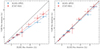 |
Fig. C.1. ALMA-only flux density measurements (Goddi et al. 2021) versus intra-site VLBI flux densities obtained during the EHT campaign, as reported in Table 2. The available data points correspond to observations of 3C279, 3C273, Centaurus A, OJ287, 1055+018, J1924-2914, Sgr A*, NRAO 530, and M87. Left panel: the dashed lines scale ALMA-only flux densities down by 0.8 (red) and 0.72 (blue), to approximately match ALMA-APEX and JCMT-SMA measurements. Right panel: after correcting for 7% ALMA VLBI losses and scaling all VLBI flux densities up by 25%, we find consistency with ALMA-only data for all the sources. |
Appendix D: Acknowledgements
We thank M. Sikora, K. Nalewajko, and A. Plavin for comments. J. Röder received financial support for this research from the International Max Planck Research School (IMPRS) for Astronomy and Astrophysics at the Universities of Bonn and Cologne. This research has made use of the SIMBAD database, operated at CDS, Strasbourg, France. This study makes use of VLBA data from the VLBA-BU Blazar Monitoring Program (BEAM-ME and VLBA-BU-BLAZAR, funded by NASA through the Fermi Guest Investigator Program). J. Röder further acknowledges financial support from the Severo Ochoa grant CEX2021-001131-S funded by MCIN/AEI/10.13039/501100011033.
The Event Horizon Telescope Collaboration thanks the following organizations and programs: the Academia Sinica; the Academy of Finland (projects 274477, 284495, 312496, 315721); the Agencia Nacional de Investigación y Desarrollo (ANID), Chile via NCN19_058 (TITANs), Fondecyt 1221421 and BASAL FB210003; the Alexander von Humboldt Stiftung; an Alfred P. Sloan Research Fellowship; Allegro, the European ALMA Regional Centre node in the Netherlands, the NL astronomy research network NOVA and the astronomy institutes of the University of Amsterdam, Leiden University, and Radboud University; the ALMA North America Development Fund; the Astrophysics and High Energy Physics programme by MCIN (with funding from European Union NextGenerationEU, PRTR-C17I1); the Black Hole Initiative, which is funded by grants from the John Templeton Foundation (60477, 61497, 62286) and the Gordon and Betty Moore Foundation (Grant GBMF-8273) - although the opinions expressed in this work are those of the author and do not necessarily reflect the views of these Foundations ; the Brinson Foundation; “la Caixa” Foundation (ID 100010434) through fellowship codes LCF/BQ/DI22/11940027 and LCF/BQ/DI22/11940030; Chandra DD7-18089X and TM6-17006X; the China Scholarship Council; the China Postdoctoral Science Foundation fellowships (2020M671266, 2022M712084); Conicyt through Fondecyt Postdoctorado (project 3220195); Consejo Nacional de Humanidades, Ciencia y Tecnología (CONAHCYT, Mexico, projects U0004-246083, U0004-259839, F0003-272050, M0037-279006, F0003-281692, 104497, 275201, 263356, 257435, CBF2023-2024-1102); the Colfuturo Scholarship; the Consejería de Economía, Conocimiento, Empresas y Universidad of the Junta de Andalucía (grant P18-FR-1769), the Consejo Superior de Investigaciones Científicas (grant 2019AEP112); the Delaney Family via the Delaney Family John A. Wheeler Chair at Perimeter Institute; Dirección General de Asuntos del Personal Académico-Universidad Nacional Autónoma de México (DGAPA-UNAM, projects IN112820 and IN108324); the Dutch Research Council (NWO) for the VICI award (grant 639.043.513), the grant OCENW.KLEIN.113, and the Dutch Black Hole Consortium (with project No. NWA 1292.19.202) of the research programme the National Science Agenda; the Dutch National Supercomputers, Cartesius and Snellius (NWO grant 2021.013); the EACOA Fellowship awarded by the East Asia Core Observatories Association, which consists of the Academia Sinica Institute of Astronomy and Astrophysics, the National Astronomical Observatory of Japan, Center for Astronomical Mega-Science, Chinese Academy of Sciences, and the Korea Astronomy and Space Science Institute; the European Research Council (ERC) Synergy Grant “BlackHoleCam: Imaging the Event Horizon of Black Holes" (grant 610058) and Synergy Grant "BlackHolistic: Colour Movies of Black Holes: Understanding Black Hole Astrophysics from the Event Horizon to Galactic Scales" (grant 10107164); the European Union Horizon 2020 research and innovation programme under grant agreements RadioNet (No. 730562), M2FINDERS (No. 101018682) and FunFiCO (No. 777740); the Horizon ERC Grants 2021 programme under grant agreement No. 101040021; the European Research Council for advanced grant ‘JETSET: Launching, propagation and emission of relativistic jets from binary mergers and across mass scales’ (grant No. 884631); the European Horizon Europe staff exchange (SE) programme HORIZON-MSCA-2021-SE-01 grant NewFunFiCO (No. 10108625); the FAPESP (Fundação de Amparo á Pesquisa do Estado de São Paulo) under grant 2021/01183-8; the Fondo CAS-ANID folio CAS220010; the Generalitat Valenciana (grants APOSTD/2018/177 and ASFAE/2022/018) and GenT Program (project CIDEGENT/2018/021); the Gordon and Betty Moore Foundation (GBMF-3561, GBMF-5278, GBMF-10423); the Institute for Advanced Study; the ICSC – Centro Nazionale di Ricerca in High Performance Computing, Big Data and Quantum Computing, funded by European Union – NextGenerationEU; the Istituto Nazionale di Fisica Nucleare (INFN) sezione di Napoli, iniziative specifiche TEONGRAV; the International Max Planck Research School for Astronomy and Astrophysics at the Universities of Bonn and Cologne; the Italian Ministry of University and Research (MUR)– Project CUP F53D23001260001, funded by the European Union – NextGenerationEU; DFG research grant “Jet physics on horizon scales and beyond” (grant No. 443220636); Joint Columbia/Flatiron Postdoctoral Fellowship (research at the Flatiron Institute is supported by the Simons Foundation); the Japan Ministry of Education, Culture, Sports, Science and Technology (MEXT; grant JPMXP1020200109); the Japan Society for the Promotion of Science (JSPS) Grant-in-Aid for JSPS Research Fellowship (JP17J08829); the Joint Institute for Computational Fundamental Science, Japan; the Key Research Program of Frontier Sciences, Chinese Academy of Sciences (CAS, grants QYZDJ-SSW-SLH057, QYZDJSSW-SYS008, ZDBS-LY-SLH011); the Leverhulme Trust Early Career Research Fellowship; the Max-Planck-Gesellschaft (MPG); the Max Planck Partner Group of the MPG and the CAS; the MEXT/JSPS KAKENHI (grants 18KK0090, JP21H01137, JP18H03721, JP18K13594, 18K03709, JP19K14761, 18H01245, 25120007, 23K03453); the MICINN Research Projects PID2019-108995GB-C22, PID2022-140888NB-C22 ; the MIT International Science and Technology Initiatives (MISTI) Funds; the Ministry of Science and Technology (MOST) of Taiwan (103-2119-M-001-010-MY2, 105-2112-M-001-025-MY3, 105-2119-M-001-042, 106-2112-M-001-011, 106-2119-M-001-013, 106-2119-M-001-027, 106-2923-M-001-005, 107-2119-M-001-017, 107-2119-M-001-020, 107-2119-M-001-041, 107-2119-M-110-005, 107-2923-M-001-009, 108-2112-M-001-048, 108-2112-M-001-051, 108-2923-M-001-002, 109-2112-M-001-025, 109-2124-M-001-005, 109-2923-M-001-001, 110-2112-M-003-007-MY2, 110-2112-M-001-033, 110-2124-M-001-007, and 110-2923-M-001-001); the Ministry of Education (MoE) of Taiwan Yushan Young Scholar Program; the Physics Division, National Center for Theoretical Sciences of Taiwan; the National Aeronautics and Space Administration (NASA, Fermi Guest Investigator grant 80NSSC20K1567, NASA Astrophysics Theory Program grant 80NSSC20K0527, NASA NuSTAR award 80NSSC20K0645); NASA Hubble Fellowship grants HST-HF2-51431.001-A, HST-HF2-51482.001-A, HST-HF2-51539.001-A awarded by the Space Telescope Science Institute, which is operated by the Association of Universities for Research in Astronomy, Inc., for NASA, under contract NAS5-26555; the National Institute of Natural Sciences (NINS) of Japan; the National Key Research and Development Program of China (grant 2016YFA0400704, 2017YFA0402703, 2016YFA0400702); the National Science and Technology Council (NSTC, grants NSTC 111-2112-M-001 -041, NSTC 111-2124-M-001-005, NSTC 112-2124-M-001-014); the US National Science Foundation (NSF, grants AST-0096454, AST-0352953, AST-0521233, AST-0705062, AST-0905844, AST-0922984, AST-1126433, OIA-1126433, AST-1140030, DGE-1144085, AST-1207704, AST-1207730, AST-1207752, MRI-1228509, OPP-1248097, AST-1310896, AST-1440254, AST-1555365, AST-1614868, AST-1615796, AST-1715061, AST-1716327, AST-1726637, OISE-1743747, AST-1743747, AST-1816420, AST-1952099, AST-1935980, AST-2034306, AST-2205908, AST-2307887); NSF Astronomy and Astrophysics Postdoctoral Fellowship (AST-1903847); the Natural Science Foundation of China (grants 11650110427, 10625314, 11721303, 11725312, 11873028, 11933007, 11991052, 11991053, 12192220, 12192223, 12273022, 12325302, 12303021); the Natural Sciences and Engineering Research Council of Canada (NSERC, including a Discovery Grant and the NSERC Alexander Graham Bell Canada Graduate Scholarships-Doctoral Program); the National Youth Thousand Talents Program of China; the National Research Foundation of Korea (the Global PhD Fellowship Grant: grants NRF-2015H1A2A1033752, the Korea Research Fellowship Program: NRF-2015H1D3A1066561, Brain Pool Program: 2019H1D3A1A01102564, Basic Research Support Grant 2019R1F1A1059721, 2021R1A6A3A01086420, 2022R1C1C1005255, 2022R1F1A1075115); the National Research Foundation of Korea (NRF) grant funded by the Korean government (MSIT) (RS-2024-00449206); Netherlands Research School for Astronomy (NOVA) Virtual Institute of Accretion (VIA) postdoctoral fellowships; NOIRLab, which is managed by the Association of Universities for Research in Astronomy (AURA) under a cooperative agreement with the National Science Foundation; Onsala Space Observatory (OSO) national infrastructure, for the provisioning of its facilities/observational support (OSO receives funding through the Swedish Research Council under grant 2017-00648);
the Perimeter Institute for Theoretical Physics (research at Perimeter Institute is supported by the Government of Canada through the Department of Innovation, Science and Economic Development and by the Province of Ontario through the Ministry of Research, Innovation and Science); the Portuguese Foundation for Science and Technology (FCT) grants (Individual CEEC program - 5th edition, https://doi.org/10.54499/UIDB/04106/2020, https://doi.org/10.54499/UIDP/04106/2020, PTDC/FIS-AST/3041/2020, CERN/FIS-PAR/0024/2021, 2022.04560.PTDC); the Princeton Gravity Initiative; the Spanish Ministerio de Ciencia e Innovación (grants PGC2018-098915-B-C21, AYA2016-80889-P, PID2019-108995GB-C21, PID2020-117404GB-C21, RYC2023-042988-I); the University of Pretoria for financial aid in the provision of the new Cluster Server nodes and SuperMicro (USA) for a SEEDING GRANT approved toward these nodes in 2020; the Shanghai Municipality orientation program of basic research for international scientists (grant no. 22JC1410600); the Shanghai Pilot Program for Basic Research, Chinese Academy of Science, Shanghai Branch (JCYJ-SHFY-2021-013); the Simons Foundation (grant 00001470); the State Agency for Research of the Spanish MCIU through the “Center of Excellence Severo Ochoa” award for the Instituto de Astrofísica de Andalucía (SEV-2017- 0709); the Spanish Ministry for Science and Innovation grant CEX2021-001131-S funded by MCIN/AEI/10.13039/501100011033; the Spinoza Prize SPI 78-409; the South African Research Chairs Initiative, through the South African Radio Astronomy Observatory (SARAO, grant ID 77948), which is a facility of the National Research Foundation (NRF), an agency of the Department of Science and Innovation (DSI) of South Africa; the Toray Science Foundation; the Swedish Research Council (VR); the UK Science and Technology Facilities Council (grant no. ST/X508329/1); the US Department of Energy (USDOE) through the Los Alamos National Laboratory (operated by Triad National Security, LLC, for the National Nuclear Security Administration of the USDOE, contract 89233218CNA000001); and the YCAA Prize Postdoctoral Fellowship.
We thank the staff at the participating observatories, correlation centers, and institutions for their enthusiastic support. This paper makes use of the following ALMA data: ADS/JAO.ALMA#2016.1.00413.V, ADS/JAO.ALMA#2016.1.01114.V, ADS/JAO.ALMA#2016.1.01116.V, ADS/JAO.ALMA#2016.1.01154.V, ADS/JAO.ALMA#2016.1.01176.V, ADS/JAO.ALMA#2016.1.01198.V, ADS/JAO.ALMA#2016.1.01216.V, ADS/JAO.ALMA#2016.1.01290.V, ADS/JAO.ALMA#2016.1.01404.V, ADS/JAO.ALMA#2017.1.00841.V, ADS/JAO.ALMA#2013.1.01022.S, ADS/JAO.ALMA#2015.1.01170.S, ADS/JAO.ALMA#2016.1.00415.S, ADS/JAO.ALMA#2017.1.00608.S. ALMA is a partnership of the European Southern Observatory (ESO; Europe, representing its member states), NSF, and National Institutes of Natural Sciences of Japan, together with National Research Council (Canada), Ministry of Science and Technology (MOST; Taiwan), Academia Sinica Institute of Astronomy and Astrophysics (ASIAA; Taiwan), and Korea Astronomy and Space Science Institute (KASI; Republic of Korea), in cooperation with the Republic of Chile. The Joint ALMA Observatory is operated by ESO, Associated Universities, Inc. (AUI)/NRAO, and the National Astronomical Observatory of Japan (NAOJ). The NRAO is a facility of the NSF operated under cooperative agreement by AUI.
This research used data obtained with the Global Millimeter VLBI Array (GMVA). The GMVA consists of telescopes operated by the MPIfR, IRAM, Onsala, Metsahovi, Yebes, the Korean VLBI Network, the Green Bank Observatory and the Very Long Baseline Array (VLBA). The VLBA and the GBT are facilities of the National Science Foundation operated under cooperative agreement by Associated Universities, Inc. GMVA data were correlated at the Max Planck Institute for Radio Astronomy (Bonn, Germany). This research used resources of the Oak Ridge Leadership Computing Facility at the Oak Ridge National Laboratory, which is supported by the Office of Science of the U.S. Department of Energy under contract No. DE-AC05-00OR22725; the ASTROVIVES FEDER infrastructure, with project code IDIFEDER-2021-086; the computing cluster of Shanghai VLBI correlator supported by the Special Fund for Astronomy from the Ministry of Finance in China; We also thank the Center for Computational Astrophysics, National Astronomical Observatory of Japan. This work was supported by FAPESP (Fundacao de Amparo a Pesquisa do Estado de Sao Paulo) under grant 2021/01183-8.
APEX is a collaboration between the Max-Planck-Institut für Radioastronomie (Germany), ESO, and the Onsala Space Observatory (Sweden). The SMA is a joint project between the SAO and ASIAA and is funded by the Smithsonian Institution and the Academia Sinica. The JCMT is operated by the East Asian Observatory on behalf of the NAOJ, ASIAA, and KASI, as well as the Ministry of Finance of China, Chinese Academy of Sciences, and the National Key Research and Development Program (No. 2017YFA0402700) of China and Natural Science Foundation of China grant 11873028. Additional funding support for the JCMT is provided by the Science and Technologies Facility Council (UK) and participating universities in the UK and Canada. The LMT is a project operated by the Instituto Nacional de Astrófisica, Óptica, y Electrónica (Mexico) and the University of Massachusetts at Amherst (USA). The IRAM 30-m telescope on Pico Veleta, Spain is operated by IRAM and supported by CNRS (Centre National de la Recherche Scientifique, France), MPG (Max-Planck-Gesellschaft, Germany), and IGN (Instituto Geográfico Nacional, Spain). The SMT is operated by the Arizona Radio Observatory, a part of the Steward Observatory of the University of Arizona, with financial support of operations from the State of Arizona and financial support for instrumentation development from the NSF. Support for SPT participation in the EHT is provided by the National Science Foundation through award OPP-1852617 to the University of Chicago. Partial support is also provided by the Kavli Institute of Cosmological Physics at the University of Chicago. The SPT hydrogen maser was provided on loan from the GLT, courtesy of ASIAA.
This work used the Extreme Science and Engineering Discovery Environment (XSEDE), supported by NSF grant ACI-1548562, and CyVerse, supported by NSF grants DBI-0735191, DBI-1265383, and DBI-1743442. XSEDE Stampede2 resource at TACC was allocated through TG-AST170024 and TG-AST080026N. XSEDE JetStream resource at PTI and TACC was allocated through AST170028. This research is part of the Frontera computing project at the Texas Advanced Computing Center through the Frontera Large-Scale Community Partnerships allocation AST20023. Frontera is made possible by National Science Foundation award OAC-1818253. This research was done using services provided by the OSG Consortium (Pordes et al. 2007; Sfiligoi et al. 2009) supported by the National Science Foundation award Nos. 2030508 and 1836650. Additional work used ABACUS2.0, which is part of the eScience center at Southern Denmark University, and the Kultrun Astronomy Hybrid Cluster (projects Conicyt Programa de Astronomia Fondo Quimal QUIMAL170001, Conicyt PIA ACT172033, Fondecyt Iniciacion 11170268, Quimal 220002). Simulations were also performed on the SuperMUC cluster at the LRZ in Garching, on the LOEWE cluster in CSC in Frankfurt, on the HazelHen cluster at the HLRS in Stuttgart, and on the Pi2.0 and Siyuan Mark-I at Shanghai Jiao Tong University. The computer resources of the Finnish IT Center for Science (CSC) and the Finnish Computing Competence Infrastructure (FCCI) project are acknowledged. This research was enabled in part by support provided by Compute Ontario (http://computeontario.ca), Calcul Quebec (http://www.calculquebec.ca), and Compute Canada (http://www.computecanada.ca).
The EHTC has received generous donations of FPGA chips from Xilinx Inc., under the Xilinx University Program. The EHTC has benefited from technology shared under open-source license by the Collaboration for Astronomy Signal Processing and Electronics Research (CASPER). The EHT project is grateful to T4Science and Microsemi for their assistance with hydrogen masers. This research has made use of NASA’s Astrophysics Data System. We gratefully acknowledge the support provided by the extended staff of the ALMA, from the inception of the ALMA Phasing Project through the observational campaigns of 2017 and 2018. We would like to thank A. Deller and W. Brisken for EHT-specific support with the use of DiFX. We thank Martin Shepherd for the addition of extra features in the Difmap software that were used for the CLEAN imaging results presented in this paper. We acknowledge the significance that Maunakea, where the SMA and JCMT EHT stations are located, has for the indigenous Hawaiian people.
All Tables
Flux densities, core sizes, and core brightness temperatures at 230 GHz measured during the 2017 EHT observing campaign.
Slopes of the power law fits obtained with different methods of fitting to data shown in Fig. 4
All Figures
|
Fig. 1. (u, v) coverage for all sources observed during the EHT 2017 campaign, as summarized in Table 1, combining all available visibility detections for all days and bands, averaged in 120 s intervals. The two circles in each panel correspond to the fringe spacing characterizing an instrumental resolution of 25 and 50 μas. JCMT-SMA and ALMA-APEX are the very short intrasite baselines, shown as black data points near the origin of the (u, v) coordinate system (when available). JCMT and SMA are shown as “Hawai’i”, while ALMA and APEX are shown as “Chile”. |
| In the text | |
|
Fig. 2. Models of the EHT sources obtained through (polarized) circular Gaussian model fitting with at least two components. Blue crosses in the left column indicate positions of individual components. Contours represent 0.1, 0.3, 0.5, 0.7 and 0.9 of the peak total intensity. EHT observing beams are shown with dashed-line ellipses, to give a sense of the diffraction limited resolution supported by the data sets. We show consistency between models (black) and data (blue) for visibility amplitudes, closure phases, and absolute values of fractional visibility polarization. Closure phases are shown as a function of combined baseline length, which corresponds to a quadrature sum of lengths of all baselines from a given triangle. The visibility domain fractional polarization may exceed unity for resolved sources, such as is the case for 1749+096. The data shown contain detections only and no upper limits. |
| In the text | |
|
Fig. 3. Core brightness temperature against core synchrotron spectral luminosity for the EHT 2017 sample of 16 AGN sources. The sources cluster into categories of radio galaxies, BL Lacs (blazars), and quasars. |
| In the text | |
|
Fig. 4. Measurements of the core flux density (top), size (middle), and brightness temperature (bottom) obtained using the EHT+ data set of AGN sources, as a function of frequency in the host frame. The 15–230 GHz ground array data in each panel are approximated by power law fits (solid lines, obtained as detailed in Sect. 3.1) and the fit results are annotated. The faded data points are the RadioAstron measurements, while regular data points at the same frequencies correspond to VLBA and VSOP measurements; for comparability, we color the 1.66 GHz (L band) RadioAstron points the same as the 2 GHz (S band) VLBA points. The slope of the core flux density is shallow, Sν ∝ ν−0.4. The core size decreases with frequency (and, in turn, increases with the distance from the central engine) as θ ∝ ν−0.6; the brightness temperature decreases with frequency as Tb ∝ ν−1.0. |
| In the text | |
|
Fig. 5. Core size (top), brightness temperature (middle), and magnetic field estimate (bottom) obtained from the EHT+ data set as a function of the distance to the central engine. The 15–230 GHz data in each panel are approximated by power law fits (solid lines, obtained as detailed in Sect. 3.1) and the fit results are annotated. The faded data points at are the RadioAstron measurements, while the filled markers correspond to VLBA observations. For comparability, we color the 1.66 GHz (L band) RadioAstron points the same as the 2 GHz (S band) VLBA points. For a M• = 108 M⊙ black hole 1 pc =2 × 10⁵rg with gravitational radius rg = GM•/c2. |
| In the text | |
|
Fig. A.1. Models of the EHT 2017 sources obtained through the fitting of linearly polarized circular Gaussians. Contours represent 0.1, 0.3, 0.5, 0.7 and 0.9 of the peak total intensity brightness, same as in Fig. 2. Blue crosses: fitted positions of the Gaussians. Color map: fractional polarization. Total flux densities Itot and total fractional polarization levels mnet for the reconstructed compact structures are annotated. |
| In the text | |
|
Fig. C.1. ALMA-only flux density measurements (Goddi et al. 2021) versus intra-site VLBI flux densities obtained during the EHT campaign, as reported in Table 2. The available data points correspond to observations of 3C279, 3C273, Centaurus A, OJ287, 1055+018, J1924-2914, Sgr A*, NRAO 530, and M87. Left panel: the dashed lines scale ALMA-only flux densities down by 0.8 (red) and 0.72 (blue), to approximately match ALMA-APEX and JCMT-SMA measurements. Right panel: after correcting for 7% ALMA VLBI losses and scaling all VLBI flux densities up by 25%, we find consistency with ALMA-only data for all the sources. |
| In the text | |
Current usage metrics show cumulative count of Article Views (full-text article views including HTML views, PDF and ePub downloads, according to the available data) and Abstracts Views on Vision4Press platform.
Data correspond to usage on the plateform after 2015. The current usage metrics is available 48-96 hours after online publication and is updated daily on week days.
Initial download of the metrics may take a while.